


1. Introduction
A cornerstone of lexical processing research for decades has been the idea that sets of words similar in form are activated together, and that the size and contents of these sets influence the course and results of processing. These sets are often referred to as neighborhoods, most commonly defined as the set of words that differ from a given target word by the substitution (Coltheart et al., 1977; Landauer & Streeter, 1973), addition, or subtraction (Luce & Pisoni, 1998) of one phoneme (phonological neighbors) or letter (orthographic neighbors).
There is now copious evidence that neighborhood density (ND, the number of neighbors a target word has) relates to auditory and visual word recognition (e.g., Andrews, 1997; Vitevitch & Luce, 2016), and all current theories account for density in some way. It has, moreover, become nearly ubiquitous as a covariate or control variable. ND effects are also well-documented in spoken (Vitevitch & Luce, 2016), signed (Caselli et al., 2021), and written (Roux & Bonin, 2009) word production, in language development (Charles-Luce & Luce, 1990, 1995; Coady & Aslin, 2003; Swingley & Aslin, 2002, 2007), in the errors made by healthy younger and older adults (Harley & Brown, 1998; Sommers, 1996; Stemberger, 2004; Vitevitch, 1997, 2002; Vitevitch & Sommers, 2003), and by individuals with developmental disabilities or neurological impairments (Goldrick et al., 2010; Storkel, 2009).
Various refinements to ND have been proposed to address theoretical and practical concerns with this measure. These include attempts to incorporate a similarity gradient beyond an edit distance of one1 (Iverson et al., 1998; Luce & Pisoni, 1998; Strand, 2014; Suárez et al., 2011; Yarkoni et al., 2008), or to compute finer gradations of similarity by incorporating subsegmental features (Bailey & Hahn, 2005; Hahn & Bailey, 2005; Strand, 2014). Others have shown that ND effects depend on other properties of neighborhoods, such as the frequencies of the target word’s neighbors (Luce & Pisoni, 1998; Vitevitch & Luce, 1998), competition from neighbors at the same segment position (McClelland & Rumelhart, 1981), and whether neighbors overlap early or later in their forms, or form a cohort (Allopenna et al., 1998; Fricke et al., 2016; Marslen-Wilson & Tyler, 1980). ND may also be conditioned on the syntactic categories of the target and its neighbors (Heller & Goldrick, 2014; Strand et al., 2014).
A different approach to examining word-form similarity structure in the lexicon builds on the idea that neighbor-to-neighbor links allow an entire lexicon to be represented as a graph (Vitevitch, 2008). A graph is a mathematical structure comprised of a set of nodes and a set of edges that connect the nodes based on some criteria. Network science studies the application of graph theory to real-world phenomena, including a recent burst of activity related to cognition (see Baronchelli et al., 2013; Siew et al., 2019, for recent reviews). In nearly all studies of phonological or orthographic networks, the nodes represent words, and edges connect words that have an edit distance of 1, i.e., neighbors. We refer to this kind of network as neighbor networks (following Brown et al., 2018).2 Networks could be built using other criteria, e.g., incorporating syllable structure (cf. Sun & Poeppel, 2023, on the role or syllables in lexical organization, though they did not use a network), or phonotactics (e.g., via biphones or a bipartite network linking phonemes to words; Vitevitch et al., 2021), or placing edges based on human misperceptions or intuitions about phonological associations (Castro & Vitevitch, 2022). However, useful alternatives to the edit distance = 1 criterion are potentially many and have not yet been systematically explored.
Neighbor networks go beyond addressing some of the weaknesses of ND (e.g., by incorporating gradient similarity by providing paths connecting words that are not immediate neighbors), but, more importantly, they implement the idea of phonological and orthographic structure in the lexicon. Network science offers a wealth of concepts and measures for quantifying the position of nodes in a network, which we will refer to as nodal properties (Bullmore & Sporns, 2009; Sporns, 2011; Vitevitch, 2008). There is growing evidence in psycholinguistics that a variety of nodal properties capture useful information about the properties of words’ immediate neighborhoods (micro-level structure), as well as complexity in the distribution and relationships among words at larger (meso- and macro-) scales and distances from the target (for a review, see Vitevitch, 2022).
The idea of word-form based structure in the lexicon has potential for opening new theoretical perspectives on how word-form similarity constrains lexical processing (Castro & Siew, 2020; Siew et al., 2019; Vitevitch, 2008, 2022), but the underlying theoretical nature of structure, as it may be measured in neighbor networks, is not yet clear, making it hard to explore that potential. There are three reasons for this. First, as noted above, useful alternatives to the edit distance = 1 criterion are potentially many and have not yet been systematically explored. Second, the nodal properties used to measure aspects of structure have precise mathematical definitions that depend on specific assumptions about how information flows in the network, given the phenomenon being modeled (Borgatti, 2005). These assumptions have guided the psycholinguistic study of new nodal properties, yielding important insights, but the paths in a lexical neighbor network are not as concrete as they are for other phenomena that may be modeled using networks, for example, person-to-person contact in a model of disease transmission. Finally, while networks suggest paths for activation to spread from word to word (Siew, 2019; Vitevitch, 2022), word recognition theories in general lack lateral spreading activation of this kind (e.g. Luce & Pisoni, 1998; Marslen-Wilson & Tyler, 1980; McClelland & Elman, 1986; McClelland & Rumelhart, 1981; Norris, 1994; Norris & McQueen, 2008; see Weber & Scharenborg, 2012, for a detailed review), and some models do not include word form representations (i.e., the network nodes) at all (Baayen et al., 2019; Shafaei-Bajestan et al., 2023).
In this article, we therefore take the documented effects of various nodal properties as evidence that the networks capture relevant aspects of phonological and orthographic structure in the mental lexicon, but we explore the usefulness of considering those measures as proxies of some set of underlying dimensions that serve to describe that structure. To gain insight into those dimensions, we apply a data-driven latent variable technique to relate a large set of nodal properties, including several that have not been explored previously, to auditory and visual word recognition data from recent mega-studies (Balota et al., 2007; Tucker et al., 2019).
In this way, we seek to shed light on what it means to say that the lexicon is structured based on phonological and orthographic word-form similarity. Theoretically, we hope that the insights gained will help narrow the gap between the notion of structure suggested by network models and word recognition theory. Methodologically, we aim to clarify the links between nodal properties and the underlying constructs they measure, contributing to our understanding of how networks can be used and interpreted in psycholinguistics.
1.1 The lexicon as a neighbor network
The first studies of neighbor networks focused on properties of the entire network. Vitevitch (2008; see also Arbesman et al., 2010a, 2010b) studied a phonological neighbor network comprising 19,340 words from the Merriam-Webster Pocket Dictionary. The largest connected component of the network, called the Giant Component (GC), contained 6,508 nodes, and there were many smaller components, including hermits (words with no neighbors). The GC itself had a high mean clustering coefficient and assortativity, and low average shortest path length. Clustering quantifies the extent to which each word’s neighbors are also neighbors of each other, and assortativity means that words and their neighbors tend to have similar degree (degree is the network science term for the number of neighbors a node has). High clustering and low average shortest path length are indicative of small-worldness (Humphries & Gurney, 2008; Watts & Strogatz, 1998).
Properties like this, found in many networks, including social, neural, and semantic networks, are thought to favor efficient flow of information (Watts & Strogatz, 1998), leading to the suggestion that lexical structure evolves to favor efficient search (Vitevitch, 2008). However, many of the topological properties of neighbor networks in several languages, including the degree distribution, the distribution of connected component sizes, mean shortest path length, clustering, and assortativity, are well approximated in random pseudolexicons generated with minimal linguistic constraints – namely, with the same word length distribution and number of phonetic categories, but with no constraints on CV structure or phonotactics (Brown et al., 2018; Gruenenfelder & Pisoni, 2009; but see Stella & Brede, 2015). Moreover, adding such constraints has little impact on the properties of the resulting pseudolexicon networks. These topological properties may, thus, be an inevitable feature of networks in which the nodes represent strings constructed from a limited set of sub-nodal units, such as words encoded as strings of letters/phonemes. Global network structure, therefore, does not provide unambiguous evidence that lexicons have evolved to favor efficient search, but structure may, nevertheless, help explain the overall efficiency of lexical processing.
The other approach to studying network structure in lexical processing is to use properties of the nodes to quantify each word’s position in the network in various ways (see Table 1, below, for a list of the nodal properties we study, and their definitions). The entire literature on neighborhood density comprises the simplest way to do this, since ND is merely the most local, or micro-level, property of nodes in a network (called degree). Research has explored new nodal properties incrementally, based on their expected effects on the flow of information through the network. This includes meso- and macro-level properties (Vitevitch, 2022), which quantify structure in progressively larger subsets of words surrounding a target (e.g., clustering, community structure), ultimately encompassing the whole network or connected component (e.g., closeness centrality, which is the average shortest path length between each target word and all other words in the component).
Table 1: Network Measures and Descriptions.
| Measure | Description |
| Degree | The number of edges connected to a node, i.e., neighborhood density. |
| Average Neighbor Degree | The average degree of each node’s neighbors. This is related to degree assortativity (Vitevitch, 2008), which is defined as the correlation between a node’s degree and the degrees of its neighbors, across all pairs of neighbors in the network. |
| Average Neighbor Frequency | The average log frequency of each node’s neighbors. This is not, strictly speaking, a property of the network itself, but of certain nodes identified based on their relationship in the network. Neighborhood density is often weighted by neighbor frequencies in the literature (Luce & Pisoni, 1998). |
| Clustering Coefficient | Proportion of pairs of a node’s neighbors that are also neighbors to each other (undefined for nodes with fewer than two neighbors). |
| Local Efficiency | A measure of the average efficiency of information transfer. Related to clustering coefficient, local efficiency of each node is the average of the inverse shortest path lengths in a subgraph comprised of the node’s neighbors (excluding the target node). |
| Coreness | The kth core consists of those nodes that remain after recursively pruning all nodes with degree < k, but are removed when recursively pruning all nodes with degree = k. Since pruning is recursive, coreness may be smaller than degree, but it cannot be greater. It measures longer-range integration or embeddedness within a network, in the sense that words with high coreness are interconnected with a set of words having equal or greater degree, such that those words survive the pruning procedure for lower values of k. Coreness in the phonological network predicts children’s vocabulary growth (Carlson et al., 2014). |
| Community Size | The number of nodes that are in a node’s community. A community is a subgraph selected to optimize modularity of the network (Siew, 2013) and consists of a set of nodes that are more densely interconnected with each other than with other (nearby) nodes. |
| Participation Coefficient | A measure of how many communities a node’s neighbors are connected to and how evenly distributed a node’s neighbors are across those communities. This has not been directly examined in relation to word recognition, but we include it based on recent work on the relevance of community structure more generally (Siew, 2013). Nodes with high participation serve as “connector hubs”, having neighbors in many communities outside of their own, and nodes with low participation tend to lack neighbors outside of their own community. |
| Within-module degree z-score | The z-score of each node’s degree, within its community. High values identify nodes that serve as “provincial hubs” within their own communities. This is also included based on its relevance to community structure. |
| Betweenness Centrality | The fraction of shortest paths between all possible pairs of nodes in the same connected component that pass through a given node. It measures the extent to which each node contributes to the efficient traversal of the network. |
| PageRank Centrality | A recursive measure that is the sum of a node’s neighbors’ PageRank centralities divided by their out-degrees (Brin & Page, 1998). Usually used for directed graphs, but also defined for undirected graphs, such as those analyzed here (Grolmusz, 2012). A measure of node importance, PageRank can be interpreted as the probability that a random exploration of the graph will lead to a given node. In semantic network research, it has been linked with spreading activation and random walk mechanisms for explaining letter fluency responses, and may reflect processes that shaped the prior probabilities of words (Griffiths et al., 2007). While this has not been studied in phonological and orthographic neighbor networks, we include it here, because spreading activation and random walks have been used to interpret the relationship between these networks and word recognition (Vitevitch, 2022). |
| Closeness Centrality | The reciprocal of the sum of the shortest distances between a node and all other nodes in the same connected component. Centrally located nodes are reachable from any point in the component via a minimum number of steps, but peripherally located nodes are more distant from some parts of the component. Reflects nodal importance for any process that can follow a shortest path, even if in parallel (Borgatti, 2005). |
| Eccentricity | The length of the shortest path between a node and the farthest node from that node, residing in the same connected component. Similar to closeness, nodes with low eccentricity are relatively close to every node in their connected component, computed via shortest paths. |
The first of these properties to attract attention was clustering, because of its contribution to the efficient transmission of information. Clustering in the phonological network is related to increased auditory (Altieri et al., 2010; Chan & Vitevitch, 2009) and visual (Yates, 2013)3 lexical decision and naming response times, and to increased speech errors (Chan & Vitevitch, 2010). According to Chan and Vitevitch, this occurs because, when clustering is low, activation from the neighbors either flows back to the target or dissipates to the rest of the network, making the target stand out. When clustering is high, neighbors pass activation among themselves, maintaining their higher activation relative to the target. They also successfully simulated the effect in a computational model with this kind of activation flow. Siew (2017) observed a similar effect on spoken word recognition, using a version of clustering that includes neighbors at a Levenshtein distance of 1 or 2 (2-hop neighborhoods). Using a slightly different way of constructing the network (words were considered neighbors only if both their phonological and orthographic representations were neighbors), Siew and Vitevitch (2019) found a negative effect of clustering coefficient, again on spoken word recognition latencies.
At a more macro level, faster auditory lexical decision responses (at least for frequent words) have been found for words with high closeness centrality, which measures how quickly a target may be reached, on average, from anywhere in the same connected component (Goldstein & Vitevitch, 2017). Faster responses are also found for keywords in repetition, identification in noise, and auditory lexical decision (Vitevitch & Goldstein, 2014). Keywords are words that link larger clusters of words together in the network, such that removing them would result in fragmentation of the network, disrupting the flow of information.
At a meso level, Siew (2013) studied communities, which are groups of words that are more tightly interconnected with each other than with other words in the same component. Words in large communities tended to be shorter, more frequent, acquired earlier, and have higher degree than words in smaller communities. Siew suggested that this grouping of words together may be relevant to lexical processing because the flow of information will tend to pool within one community, which may help explain phonotactic probability effects, because words in the same community tend to share similar sound sequences. Finally, at the scale of the whole network, Siew and Vitevitch (2016) found that spoken words located in islands (smaller connected components that are not linked to the GC) were recognized and recalled more quickly and accurately than words located in the GC.
Siew (2018) brought some of these measures together in a large-scale analysis of visual lexical decision and word naming data for 11,358 words from the English Lexicon Project (Balota et al., 2007). Siew found that degree was associated with decreased response latencies (contrary to many, though not all, published studies; see the review by Vitevitch & Luce, 2016) and higher accuracy in both lexical decision and word naming. A high clustering coefficient was associated with longer response latencies and marginally lower accuracy in lexical decision, and high closeness centrality was associated with faster lexical decision responses, and with slower and less accurate naming responses. These three variables together accounted for an increase in R2 of a little under 1%, over a model including lexical frequency and length in letters, phonemes, and syllables. Despite these apparently small effects, these results provide evidence that network-like structure in the mental lexicon at various scales, regarding phonological or orthographic word forms, influences processing.4
The link between these nodal properties and information flow has led to successful simulations of the clustering, giant component membership, and keyword effects reviewed above (Chan & Vitevitch, 2009; Siew & Vitevitch, 2016; Vitevitch & Goldstein, 2014), using computational models in which activation spreads from word to word by traversing the edges between neighbors. These models can vary in how this takes place, e.g., whether some activation remains behind as it spreads (duplication), and whether a decay function is applied (Siew, 2019; Vitevitch et al., 2011; Vitevitch & Mullin, 2021), and other processes that exploit the network’s edges, such as random or (semi-) directed search, could be substituted for spreading activation in variants of this model (Vitevitch, 2022). Other kinds of network flow, and other network structures, are currently being explored (Castro & Vitevitch, 2022; Vitevitch et al., 2021), and the inclusion of processes operating outside (e.g., governing where search begins), as well as within, networks is also possible (Hills & Kenett, 2022).
1.2 Interpreting nodal property effects on word recognition
The studies reviewed above support the conclusion that neighbor networks capture psycholinguistically important structural features of the mental lexicon, but it is not immediately clear how this should be interpreted. As noted above, the relevance of nodal properties depends on specific assumptions about information flow, given a specific kind of network structure (Borgatti, 2005). However, only a few simulations explicitly incorporate neighbor network structure of the kind used in the vast majority of the network science-based literature on word recognition, with information flowing via word-to-word activation spread over the network’s edges (Chan & Vitevitch, 2009; Siew & Vitevitch, 2016; Vitevitch & Goldstein, 2014).
In most models, including models with distributed representations, words are activated via some feed-forward or interactive activation process that links phonetic and lexical units, often incrementally (e.g., Luce et al., 2000; NAM, Luce & Pisoni, 1998; TRACE, McClelland & Elman, 1986; IAM, McClelland & Rumelhart, 1981; Norris, 1994). These models can also be viewed through a network science lens, with varying assumptions about networks’ architecture and information flow. The bipartite network of Vitevitch et al. (2021) is one example, with edges between phonological units and words, rather than between words (which Vitevitch et al. suggest may help account for effects of phonotactic probability). The NAM (Luce & Pisoni, 1998) also links different levels of representation. Word decision units monitor activation of acoustic-phonetic patterns, top-down information about word likelihoods, and the overall level of activity among decision units, with competition arising from the activation of decision units for multiple candidates at once. TRACE (McClelland & Elman, 1986) uses interactive links between phonological and lexical units (like Vitevitch et al.’s bipartite network), plus inhibitory links between competitors as a mechanism for resolving competition, where competitors are words that are simultaneously active, but need not be neighbors, strictly speaking. Some models, such as the more recent Shortlist-B (Norris & McQueen, 2008) or LDL-AURIS (Shafaei-Bajestan et al., 2023), do not directly implement network-like structure, lacking not only direct edges between word-form representations, but also explicit word-form (e.g., phonolexical) representations themselves. In Shortlist-B, words are identified by evaluating their posterior probabilities, given the phonetic representation of the incoming speech, and in LDL-AURIS, semantic representations are computed directly from acoustic or other low-level phonetic representations.
This diversity of network structures and assumptions about information flow indicates a need for care when interpreting results obtained using specific network architectures and assumptions about information flow, such as are found in the psycholinguistic literature using neighbor networks. This leads us to ask whether structure at different scales in this kind of network should be thought of as reflecting variability in the configuration and evolution of sets of candidate words during processing, such that words’ nodal properties in neighbor networks might be better interpreted as proxies for latent dimensions of structure. As an example of this thinking, Yarkoni et al. (2008) propose that findings of both inhibitory and facilitatory effects of ND in visual word recognition might be reconciled in a two-stage process in which a set of candidates become active quickly, based on the phonetic units being perceived, followed by a later inhibitory effect arising through competition between the target and specific, highly similar words.
Similarly, Yates (2013) interprets the effect of clustering in the phonological lexicon on visual word recognition through interactive activation between phonetic and lexical units (note that his study crossed modalities, although the interpretation would seem to apply regardless of modality). He argued that feedback to the phonetic units reinforces a target’s neighbors more strongly when clustering is high, because the neighbors overlap more consistently, with the differences occurring in limited positions – i.e., clustering is interpreted as a proxy measure of this consistency. They therefore remain more active relative to the target. This can explain the effects of clustering on visual word recognition, because strongly active neighbors are associated with inhibitory effects, and weakly active neighbors with facilitation (Chen & Mirman, 2012).
Interestingly, Chan and Vitevitch (see also Vitevitch & Mullin, 2021) failed to reproduce the effects of phonological clustering on auditory word recognition in simulations using computational implementations of models using interactive activation (TRACE, McClelland & Elman, 1986; jTRACE, Strauss et al., 2007) and bottom-up activation (Shortlist, Norris, 1994), but this could be due to peculiarities in the computational implementation of the models (e.g. the phonetic units, size of the lexicon, and lexicon copying procedure used in TRACE), and not necessarily to the underlying mechanisms.
1.3 The present study
In light of the foregoing, structure may be interpreted as a complex distribution of words in phonological or orthographic similarity space, leading to differences in how groups of related words participate over the course of word recognition. While networks provide many ways of measuring that structure, they do not tell us what underlying features or dimensions would suffice for describing that structure as it relates to word recognition. Our goal in the present study is to explore those underlying dimensions, shedding light on what it means to say that the mental lexicon is structured based on phonological and orthographic word forms, and what it means for that structure to influence processing.
Note that while our goal is to help work towards better explanatory models by refining our understanding of structure in the lexicon and its relationship to processing, our methods have much in common with predictive modeling and machine learning, in that we apply dimension-reduction techniques to a large pool of variables, including several nodal properties that have not yet been studied directly. The link between our methods and our longer-term explanatory goals is the theoretical construct of structure in the lexicon, and the use of neighbor networks as models of that structure. Based on this view, our latent variable approach provides a data-driven way to determine not only what measures of structure are predictive of performance in psycholinguistic tasks, but, principally, what underlying, latent constructs are useful for describing phonological and orthographic structure in the lexicon. Our work thus complements the prior literature, which has sought to determine which measures are useful in psycholinguistics by choosing nodal properties that reasonably match existing constructs (like neighborhoods) and testing them experimentally.
2. Methods
2.1 Network construction
To construct our networks, we began with the 79,672 real words in the English Lexicon Project database (ELP; Balota et al., 2007), minus words lacking phonetic transcriptions and retaining only words with HAL or SUBTLEX frequencies greater than zero (which eliminated many acronyms, misspellings, and other anomalous items). This left 70,741 real words. Within this lexicon, the ELP identifies a subset of 40,481 words (40,398 with phonetic transcriptions) based on further screening for obvious nonwords, misspellings, alternate spellings, and so forth, for which lexical decision and naming data are available (see Balota et al., 2007, for details). This subset is approximately the basis for the orthographic network used by Siew (2018), who considered it an adequate reflection of the vocabulary of an average English speaker (about 15,000 word families; Brysbaert et al., 2016).
For the present study, we follow Siew (2018), constructing networks using the 40,398 words for which behavioral data and phonetic transcriptions are available in the ELP.5 However, since this subset excluded many, mainly derived, words that would be familiar to an educated English speaker, we repeated our analyses using networks incorporating the larger set of 70,741 words with frequencies greater than zero. The results did not differ substantially, and the code, networks, data, and results from the larger networks are available in the online materials.
We note that both of these lexicons include many inflected forms, among them plural nouns, past tense verbs, along with participles, and so forth. While we are by no means the first to include inflected forms (e.g., Siew, 2018), many of the earlier studies used dictionaries, which lack inflected forms (Vitevitch, 2008). Though inflection clearly impacts neighbor network structure (at least in English, where many inflections are also neighbors), the issue of morphological relationships in phonological and orthographic networks has not yet been examined closely. We consider the inclusion of inflected words to be reasonable, based on substantial data and theory supporting the storage of regular inflected forms in memory (e.g., Bybee, 2006; Hay & Baayen, 2005; Jackendoff & Audring, 2020). Eventually, of course, a more sophisticated network structure, such as multilayer networks (see Section 4), would be needed to capture both phonological/orthographic and morphological structure. For now, since our focus is on spoken and written word recognition, we include inflected word forms.
To reflect both the auditory and visual modalities, we built two different networks, with the nodes representing the phonological and orthographic word forms, respectively. We use separate networks for two reasons. First, the literature has generally studied auditory and visual word recognition separately, and there is good reason to think that word recognition unfolds somewhat differently in each modality. Second, while there is also value to a more generalized view, there are many ways to incorporate both modalities into the same network (e.g., using multilayer networks, or drawing edges only between words that are neighbors in both modalities), and the literature to date offers no guidance for how to do this (the only example we are aware of is Siew & Vitevitch, 2019, who take the latter strategy). We therefore focus on the latent dimensionality of structure in unimodal networks, leaving the question of representing multi-modal structure for future research. Nevertheless, as described below, we incorporate both modalities into the same statistical analysis.
The phonological forms were taken from the ELP, which uses a transcription like X-SAMPA (Wells, 1997; www.phon.ucl.ac.uk/home/sampa). To prepare these phonological transcriptions for network construction, stress and syllable boundaries were removed, and digraphs were replaced to ensure a 1:1 relationship between characters and phonemes. After collapsing homophones into a single node (homographs were already represented only once in the ELP, but some homophones with different spellings were present) the unique pronunciations/letter strings served as the labels for the nodes in the phonological and orthographic networks, respectively. This procedure resulted in a phonological network containing 38,982 nodes, and an orthographic network containing 40,398 nodes.
In both networks, edges were placed between two nodes if the Levenshtein edit distance (Levenshtein, 1966) between their labels equaled 1, i.e., the insertion, deletion, or substitution of a single letter or phoneme. Consistent with previous research, this led to a Giant Component (GC) and several smaller island components, along with many hermits. The GC in the phonological network comprised 13,396 words (34% of the network), and 11,358 words (28%) in the orthographic network.
2.2 Network measures
We analyzed 13 nodal properties, listed in Table 1 with brief definitions. For purposes of exposition, we organize the table roughly from the most local to the most global properties (cf. micro, meso, and macro level structure; Vitevitch, 2022), although this should not be taken as a principled ordering. We selected these variables based on their use in prior research on lexical networks (degree, clustering, coreness, closeness centrality, and community structure) and for their potential relevance given spreading activation, random walk, or other processes suggested in the literature (such as the idea of dense attractor basins; Yarkoni et al., 2008). Our criteria for inclusion were liberal, based on our holistic approach to networks as models of structure in the lexicon, with the expectation that measures with little relevance to word recognition will show little relationship to the behavioral data. Where specific measures have not yet been used in word recognition research, we comment briefly in the table about their expected relevance.
The MATLAB (MATLAB, 2010) native function “centrality” was used to calculate degree, betweenness centrality, closeness centrality, and PageRank centrality. Average neighbor degree and frequency were computed in MATLAB. The MATLAB native function “conncomp” was used to determine each node’s connected component and its corresponding component size. The Brain Connectivity Toolbox (BCT; Rubinov & Sporns, 2010) was used to calculate eccentricity, coreness, local efficiency, and clustering coefficient. The Louvain community detection method (Blondel et al., 2008) was applied in a custom Python program that employed the NetworkX (https://pypi.org/project/networkx/) and python-Louvain (https://github.com/taynaud/python-louvain) libraries to determine the modules in the phonological network (30,783 modules, with modularity Q = 0.86) and the orthographic network (34,165 modules; Q = 0.81). Using the module information, the participation coefficient and within-module degree z-score of each node were calculated using a BCT script. The bivariate relationships of all nodal properties with the dependent variables were assessed visually, and only betweenness showed any evidence of nonlinearity or potentially influential extreme values. To remedy this, betweenness was log-transformed.
Before proceeding further, we explored the correlations among the nodal properties, both as a first approximation to how they may group together, and to assess multicollinearity. This was done using the subset of 6,457 words used in the analysis of the behavioral data described below. The bivariate correlations for nodal properties in the phonological network are shown in Table 2. The pattern of correlations in the orthographic network is similar (see the online materials).
Table 2: Bivariate correlations between nodal properties (in the phonological network) in the sample of words to be analyzed in the SCGLR.
| degree | coreness | av Neigh Degree | av Neigh Frq | clustering | efficiency | closeness | between | PageRank | eccentricity | community Size | participation | |
| coreness | .93 | |||||||||||
| av Neigh Degree | .87 | .93 | ||||||||||
| av Neigh Frq | .44 | .50 | .55 | |||||||||
| clustering | –.03 | .10 | .10 | .07 | ||||||||
| efficiency | .04 | .15 | .16 | .10 | .98 | |||||||
| closeness | .77 | .79 | .86 | .50 | –.07 | –.02 | ||||||
| between | .53 | .44 | .39 | .17 | –.56 | –.50 | .47 | |||||
| PageRank | .45 | .27 | .10 | –.01 | –.27 | –.23 | .16 | .54 | ||||
| eccentricity | –.62 | –.65 | –.73 | –.44 | .08 | .03 | –.91 | –.41 | –.11 | |||
| community Size | .09 | .07 | .10 | –.02 | –.02 | –.01 | .09 | .09 | .05 | –.07 | ||
| participation | .40 | .39 | .45 | .24 | –.25 | –.23 | .59 | .34 | .09 | –.53 | –.10 | |
| wMDZscore | .82 | .75 | .63 | .31 | .03 | .07 | .48 | .51 | .54 | –.38 | .00 | .07 |
-
Note. Correlations were computed over only the 6,457 words included for analysis of the behavioral data. Abbreviations: avNeighFrq: average neighbor frequency, avNeighDegree: average neighbor degree, between: betweenness centrality, closeness: closeness centrality, clustering: clustering coefficient, efficiency: local efficiency, PageRank: PageRank centrality, participation: participation coefficient, wMDZscore: within-module degree z-score. Significance is not noted (nearly all were significant), because of the large sample size. We focus on the strength of the correlations instead.
The most extensive relationships among these predictors are the strong positive correlations between degree, coreness, average neighbor degree, and closeness centrality, which are all negatively related to eccentricity. Degree and coreness are related by definition (such that coreness cannot exceed degree), and the positive correlation between degree and average neighbor degree corresponds to the definition of assortative mixing by degree, which is a well-documented property of phonological networks (Arbesman et al., 2010b). All three of these variables, in turn, are positively related to closeness and negatively related to eccentricity: words with many and well-connected neighbors tend to be reachable from anywhere within the connected component via comparatively short paths, nodes on the periphery are not. Other patterns are observable here, but they are described in detail with the results of the SCGLR modeling below. For the moment, these observations suggest that the relationships among nodal properties are consistent with the idea that the position of a node in the network may be describable using a smaller number of dimensions, although individual nodal properties may also make unique contributions.
2.3 Behavioral data and dependent measures of lexical processing
We tested the nodal properties and covariates (described below) against behavioral data from the ELP (Balota et al., 2007) and the MALD (Tucker et al., 2019) databases, representing visual lexical decision (ELP), word naming (ELP), and auditory lexical decision (MALD).6 We used the by-item mean response times from these mega-studies, inverse-transformed (and multiplied by –1000) to approximate normal distributions, as confirmed by visual inspection of quantile-quantile plots. While Siew (2018) also found effects on response accuracy in the ELP, accuracy was generally near ceiling, with low variability, so we omitted it. These mega-studies provide a large data set against which to test how effects of network-derived properties compare across different task conditions, and how they scale up to a more representative lexicon, in contrast to the small and more uniform word sets used in many psycholinguistic experiments.
While the phonological and orthographic networks included 38,982 and 40,398 words, respectively, analysis of the behavioral data was performed on only a subset of these data, comprising 6,457 words selected based on the following criteria. First, since several nodal properties are undefined when computed across disconnected components (e.g., closeness centrality cannot include shortest paths for pairs of nodes between which no path exists), only words residing in the GC of both networks were included (reducing the target word list to 7,026), consistent with most studies of lexical networks (but see Siew & Vitevitch, 2016). Second, only words with more than one neighbor, in both networks, were included (leaving 6,461 words), because clustering is undefined for words with only one neighbor (the denominator is the number of pairs of neighbors, but where there is only one neighbor, there are zero pairs). Finally, we included only words with RTs available in both the ELP and MALD (Tucker et al., 2019) and for which all covariates were available.
2.4 Supervised Component Generalized Linear Regression (SCGLR)
SCGLR (Bry et al., 2013; Mortier et al., 2015; Tomaschek et al., 2018) is a regression technique well-suited to data sets with many correlated predictors. It works by reducing the data to a smaller number of orthogonal components, like other latent variable techniques, but unlike other techniques, it seeks an optimal partitioning of the predictors with respect to their relationships with one or more dependent variables (DV). SCGLR, therefore, resembles Principal Components Regression, a two-step technique in which the predictors are first reduced to a smaller number of principal components based only on shared variance among the predictors (using Principal Components Analysis), and then the selected components are used to predict the dependent variable (using multiple regression). SCGLR combines these two steps into one, jointly modeling the predictors and one or more dependent variables in one step by maximizing a function based both on the shared variance among the predictors (like PCA) and on the relationship of the components with one or more dependent variables (like regression).
Since we are not merely interested in the interrelatedness of words’ network-based properties, but rather in how measures of network structure relate to lexical processing, these features make SCGLR ideally suited to our goals. Where several predictors bear a strong joint relationship to the dependent variables, groups of predictors and outcomes will load together on selected components, and where individual predictors relate uniquely to dependent variables, selected components will have loadings from those predictors. The importance of individual predictors is also estimated through standardized regression coefficients that are shrunk to account for multicollinearity, but we stress here that our goal is not to “deal with” collinearity for the purpose of identifying predictors’ unique contributions. We take a different approach to multicollinearity, allowing for the possibility that it may be more enlightening to focus on what the predictors have in common than to seek what independent contributions they may make (Morrissey & Ruxton, 2018). When we sidestep collinearity, either through stimulus design or through stepwise regression techniques,7 we focus on the portion of variance that one variable does not share with the correlated variable(s), but it may not be clear whether these unique contributions should be interpreted as evidence of an independent underlying construct, or whether it indicates different strengths and weaknesses of correlated predictors as measures of the same underlying, latent construct. An additional advantage of our approach, applied to large-scale data, is that it avoids several difficulties with using controlled subsets of items for testing. Specifically, controlling for many variables (if this can even be achieved; Cutler, 1981) is unlikely to yield representative samples of words, compromising ecological validity, and the matching of small item lists based on inherently continuous variables can lead to inconsistent and sample-dependent results (Liben-Nowell et al., 2019).
By estimating the joint variance components among the predictors that are most useful for predicting behavioral data, SCGLR is, thus, consistent with our goal of exploring what underlying dimensions of phonological and orthographic structure in the mental lexicon are psychologically relevant, and how well those dimensions are measured by the various nodal properties made available through using neighbor networks as models of structure. This data-driven approach complements the existing literature by helping to identify the underlying constructs that can link network models to theories of word recognition, helping to reconcile these mathematical models (networks) with the theoretical construct of structure in the mental lexicon.
2.5 Data analysis
SCGLR models were fit to the 6,457 words residing in the GC of both networks, and meeting the other criteria outlined above, using the SCGLR package in R (Mortier et al., 2015; R Core Team, 2023). Since SCGLR supports the simultaneous fitting of multiple dependent variables, all three DVs were included (visual lexical decision and naming latencies from the ELP, and auditory lexical decision latencies from the MALD, inverse-transformed, as described above). We included both modalities in the same analysis in order to gain insight into both the commonalities and differences in how phonological and orthographic structure in the lexicon relates to word recognition. Since SCGLR partitions the common and unique variance among the dependent variables and relates this to the partitioning of the predictors, relationships that are common to both modalities, as well as those unique to one or the other, should be captured in the fitted model. Some of the covariates we include are expected to confirm this. For example, the initial phoneme is unlikely to affect RTs to written stimuli made by button press, but it should be related to RTs measured by voice key (naming), and possibly also RTs to auditory stimuli. This expectation was borne out in the results (see below and the online materials), confirming that the model is indeed capturing this kind of subtlety. We also validated this approach by fitting separate models to visual lexical decision (with predictors from the orthographic network) and auditory lexical decision (with predictors from the phonological network). The results were very similar to the patterns reported here in the combined model, and they are presented and discussed in the online materials.
The network-derived predictors (see Table 1), and their treatment, as described above, were drawn from both the phonological and the orthographic networks. We also included several covariates, based on their well-known effects on behavioral measures of lexical processing. Frequency of the orthographic wordform (Lund & Burgess, 1996),8 length in phonemes, letters, and syllables, phonotactic probability (mean bigram frequency), and semantic neighborhood density (semND) were retrieved from the ELP database. Orthographic and phonological uniqueness points (UPs) were retrieved from the Massive Auditory Lexical Decision database (MALD; Tucker et al., 2019), along with the durations, in milliseconds, of the stimuli used in the MALD mega-study. UPs in the MALD are defined as the letter/phoneme position at which each word is distinguishable from all others, with the first letter/phoneme being at position 1. Words that cannot be uniquely identified at the last letter/phoneme (e.g. cat, which cannot be distinguished at position 3 from category) have UPs one more than the word length, (i.e., the word boundary). Thus, the uniqueness point for cat would be 4. To approximate normal distributions, frequency and the measures of word length were log-transformed, and the auditory stimulus durations were inverse-transformed; the transformations were selected based on visual inspection of quantile-quantile plots. Finally, we added a set of five dummy-coded variables encoding the initial phoneme, because amplitude-triggered voice keys, such as that used in the ELP megastudy, are affected by the acoustic properties of the initial sound. Based on the results of prior investigations into this issue (Kessler et al., 2002; Rastle & Davis, 2002; Vitevitch & Luce, 1998), these variables encoded whether the initial phoneme was (a) a vowel, (b) an obstruent, (c) a voiced obstruent, (d) a posterior consonant (/g, k, h/), and (e) an /s/ followed by another obstruent (note that sonorants are identified as phonemes that are neither vowels nor obstruents). All variables, including the dependent variables, were standardized, other than the categorical, dummy-coded predictors. All code and data, and additional details are available in the online materials.
Several steps taken to establish the validity of the results are reported in the online materials. In these, we compared the fitted response times from our model with published by-item mean RTs from two prior studies (Andrews, 1992; Siew & Vitevitch, 2016), and we refit the model using various subsets of the lexicon that more closely resemble the words used in psycholinguistic studies on network-based lexical properties, including short words, low-frequency words, and the published item lists from Vitevitch and Luce (1998, 1999), Siew and Vitevitch (2016), and Andrews (1992). Overall, these steps supported the validity of our model.
3. Results
3.1 Supervised components
SCGLR, like other latent variable techniques, reduces the dimensionality of a set of related variables, with the added feature of incorporating the relationships between latent dimensions (supervised components, sc) and a set of DVs. The number of components needed to effectively model the data was determined by minimizing the Bayesian Information Criterion using 10-fold cross-validation (Mortier et al., 2015), indicating that 8 components were sufficient. We then re-fit the SCGLR model using eight components. This model accounted for 38% of the variance (r2) in visual LDT latencies, 32% in word naming latencies, and 13% in auditory LDT latencies.
We begin by exploring how the variance in the predictors and DVs is partitioned across the 8 components via the squared correlation loadings, shown in Table 3. The squared correlation loadings represent the proportion of variance that is shared between each variable and each component, showing which groups of predictors are most related to each component. The best plane indicates the pair of components most strongly related to each variable, and best value is the proportion of variance in each variable accounted for by the best plane.
Table 3: Squared Correlation Loadings of Predictors and Dependent Variables.
| sc1 | sc2 | sc3 | sc4 | sc5 | sc6 | sc7 | sc8 | best plane | best value | |
| Dependent Variables | ||||||||||
| ldt_ELP | .38 | .12 | .10 | .28 | — | .09 | — | — | 1/4 | .66 |
| nmg_ELP | .58 | — | .09 | .15 | — | — | — | .07 | 1/4 | .73 |
| ldt_MALD | .20 | .06 | .11 | .17 | .09 | — | .27 | .09 | 1/7 | .47 |
| Predictors | ||||||||||
| ph_degree | .70 | — | — | .12 | — | — | — | — | 1/4 | .83 |
| ph_avNeighDegree | .71 | .06 | — | — | — | — | — | .08 | 1/8 | .79 |
| ph_coreness | .71 | — | — | .07 | — | — | — | .06 | 1/4 | .78 |
| ph_closeness | .69 | — | .08 | — | — | — | — | — | 1/3 | .77 |
| or_length | .69 | — | — | — | — | — | — | — | 1/3 | .74 |
| or_degree | .65 | — | — | .09 | .08 | — | — | — | 1/4 | .74 |
| or_avNeighDegree | .64 | .07 | — | — | — | — | — | — | 1/2 | .71 |
| or_closeness | .63 | — | .07 | — | .08 | — | — | — | 1/5 | .71 |
| or_coreness | .64 | — | — | .07 | — | — | — | — | 1/4 | .70 |
| ph_length | .66 | — | — | — | — | — | — | — | 1/6 | .70 |
| obstruent_initial | — | — | — | — | — | .61 | — | — | 3/6 | .64 |
| ph_eccentricity | .51 | — | .11 | — | — | — | — | .06 | 1/3 | .62 |
| ph_clustering | — | .43 | .15 | — | .18 | — | .08 | — | 2/5 | .62 |
| or_clustering | — | .42 | .19 | — | .17 | — | .07 | — | 2/3 | .61 |
| or_efficiency | — | .41 | .19 | — | .16 | — | .08 | .06 | 2/3 | .61 |
| ph_efficiency | — | .42 | .15 | — | .18 | — | .08 | .06 | 2/5 | .60 |
| ph_wMDZscore | .42 | — | .10 | .16 | — | — | — | — | 1/4 | .58 |
| freq | .28 | .09 | .16 | .27 | — | — | — | — | 1/4 | .55 |
| or_UP | .44 | .10 | — | — | — | — | — | — | 1/2 | .54 |
| V_initial | — | — | — | .09 | — | .44 | — | — | 4/6 | .53 |
| ph_UP | .42 | .09 | — | — | — | .06 | — | — | 1/2 | .51 |
| or_wMDZscore | .32 | — | .17 | .19 | — | — | — | — | 1/4 | .51 |
| or_between | .24 | .26 | — | — | .22 | — | — | — | 1/2 | .50 |
| nSyll | .38 | — | .12 | — | — | — | — | — | 1/3 | .50 |
| ph_between | .27 | .22 | — | .13 | .12 | — | — | — | 1/2 | .49 |
| or_eccentricity | .39 | — | .10 | — | .06 | — | — | — | 1/3 | .49 |
| semND | .19 | .12 | .17 | .30 | — | — | — | — | 1/4 | .49 |
| ph_participation | .22 | — | .20 | — | — | — | — | — | 1/3 | .42 |
| ph_avNeighFrq | .35 | — | — | .06 | — | — | — | .07 | 1/8 | .42 |
| sObstruent_initial | — | — | — | — | — | .06 | .29 | .13 | 7/8 | .42 |
| dur_MALD | .17 | — | — | — | .06 | — | .21 | — | 1/7 | .38 |
| or_avNeighFrq | .27 | — | — | .09 | — | — | — | — | 1/4 | .36 |
| ph_PageRank | .09 | .21 | — | .14 | — | — | — | — | 2/4 | .34 |
| or_PageRank | .08 | .22 | .06 | .08 | .07 | — | — | — | 1/2 | .30 |
| or_participation | .19 | — | .10 | — | .08 | — | — | — | 1/3 | .30 |
| voicedObs_initial | — | — | — | — | — | .15 | .15 | .11 | 6/7 | .30 |
| posterior_initial | — | — | — | — | — | .14 | .08 | — | 6/7 | .22 |
| meanBG | .06 | — | .14 | — | — | — | — | — | 1/3 | .20 |
| ph_communitySize | — | — | — | .07 | — | — | — | .08 | 4/8 | .15 |
| or_communitySize | .06 | — | — | — | — | — | — | — | 1/7 | .12 |
-
Note. Variables are sorted in descending order by their best value. Empty cells (“—”) indicate correlation loadings less than .05.
The sc1/sc4 plane, thus, captures the bulk of the relationship between the DVs and the nodal properties. This is the best plane for visual LDT and naming RTs. The best plane for auditory LDT is sc1/sc7, but its next strongest loading is on sc4, and sc7 primarily captures the effects of covariates that are most relevant to this particular task (duration of the MALD stimuli and their initial phonemes). The squared correlation loadings of the DVs on the remaining components are much smaller.
Among the predictors, most of the nodal properties and several covariates load substantially on sc1, including degree, coreness, average neighbor degree, closeness, and eccentricity, along with length-related variables and uniqueness points. This component accounted for 30% of the common variance (i.e., inertia) among the predictors (more than three times higher than the inertia of the next component). Most of these share sc1/sc4 as their best plane, like the DVs, but only frequency and semND load substantially on sc4. A largely different set of nodal properties loads more strongly on sc2, sc3, and sc5, comprised primarily of clustering, efficiency, and PageRank, but also including betweenness, participation and wMDZscore, which also load on sc1. The only variables loading substantially on sc6-sc8 are those encoding the initial phoneme and the duration of the MALD stimuli, so we do not comment further on these components.
To examine how these groups of predictors relate to the DVs, we plot the correlation loadings for several planes in Figures 1 and 2, respectively. The correlation loadings on the two components in these planes are the coordinates of each vector in these plots, and they are not squared (as in Table 3), so that the directions of the effects may be seen. The length of each vector represents the strength of the joint correlation between one predictor and the two components represented on the x and y axes (only predictors with a joint correlation loading with absolute value greater than .5 are shown). Vectors that are nearly parallel represent variables that are strongly correlated with each other on the plane. Variables that are negatively correlated with each other point in opposite directions. Other planes are available in the Plots folder in the online materials, and the code and data are also available there for further exploration.
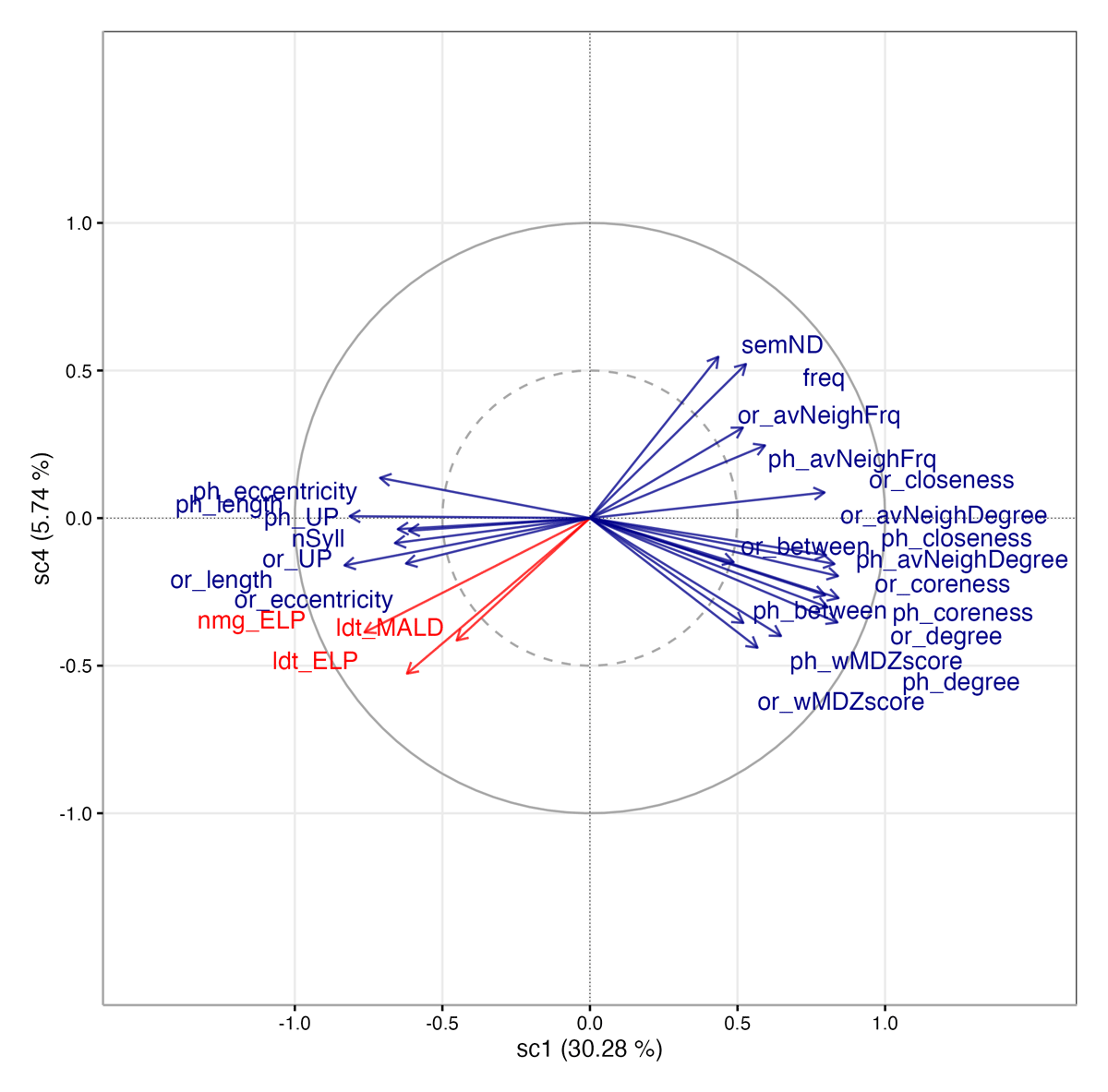
Figure 1: Correlation Loadings on the sc1/sc4 Plane. The solid circle indicates the maximum correlation (i.e., ±1), and the dotted circle indicates a correlation of ±.5. Dependent variables are labeled in red, and predictors in blue. The numbers in parentheses along each axis represent the proportion of common predictor variance accounted for by each component (i.e., inertia).
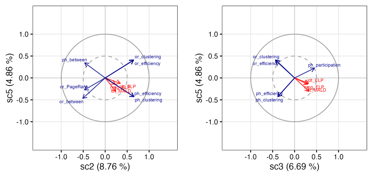
Figure 2: Correlation Loadings on the sc2/sc5 and sc3/sc5 Planes.
To begin interpreting the sc1/sc4 plane (Figure 1), note that all three DVs align closely with each other in the third quadrant, with frequency, semND, and the average neighbor frequency measures aligned more or less opposite the DVs, in the first quadrant. This indicates that this plane captures a negative relationship between shared variance among these four predictors, and shared variance among all three DVs. That is, frequent words with many semantic neighbors, and with frequent phonological and orthographic neighbors, are responded to more quickly on these tasks than infrequent words with few semantic neighbors and infrequent phonological and orthographic neighbors.
The bundle of predictors that primarily load on sc1 is also clearly seen here. Pointing to the left are length in phonemes, letters, and syllables, UPs, and eccentricity, and pointing to the right are degree, coreness, average neighbor degree, closeness, betweenness, and wMDZscore (the latter two loading somewhat more negatively on sc4). The angle between this bundle and the DVs shows that this complex of variables also explains variance in the behavioral data, with short words residing in dense areas of the lexicon associated with faster RTs.
As noted above, betweenness, wMDZscore, and participation differ from the other predictors loading on sc1 in that they also load on sc2, sc3, and/or sc5. Sc2 differentiates betweenness from the other variables in this bundle, where it shares variance with PageRank and semND, together relating negatively to the DVs. Sc3 differentiates wMDZscore and participation from the main sc1 bundle, with participation loading positively, along with the DVs on sc3, and wMDZscore loading negatively (planes sc1/sc2, and sc1/sc3, showing these patterns more directly, are available in the online materials).
Clustering, efficiency, and PageRank load on sc2, sc3, and sc5, but not on sc1. Figure 2 shows the sc2/sc5 and sc3/sc5 planes. On these planes, we can see that sc2 captures common variance involving clustering, efficiency, betweenness, and PageRank (phonological PageRank loads similarly to betweenness on sc2/sc5, but more weakly), and sc3 captures common variance in clustering, efficiency, and participation (orthographic participation loads positively on sc3 and negatively on sc5, but relatively weakly, and is not shown). Note that participation loads opposite wMDZscore on sc3, though weakly. Sc5 differentiates these variables, based on the modality of the network. Interestingly, these planes show a positive relationship between the DVs and phonological clustering/efficiency, and a negative relationship with orthographic clustering/efficiency (the lengths of the DV vectors show that these relationships are relatively weak).
3.2 Regression coefficients
To explore the overall contributions of individual predictors, we turn our attention to their standardized regression coefficients, for each DV. Unlike ordinary and mixed effects regression, where multicollinearity can lead to unreliable coefficient estimates, SCGLR shrinks the coefficients to account for the collinearity, making them interpretable (Tomaschek et al., 2018). Note, however, that they must still be interpreted in the context of the whole model, including their loadings on the supervised components, as we discuss below. Perhaps more importantly, the standardized regression coefficients allow comparison of the relative effect sizes to gauge predictors’ importances. A caterpillar plot of the standardized regression coefficients is given in Figure 3.
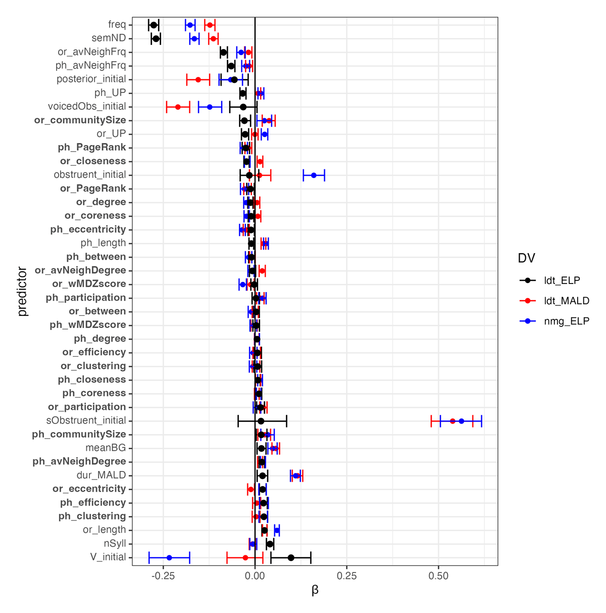
Figure 3: Standardized Regression Coefficients. The predictors are ordered, top to bottom, from the largest negative to the largest positive effect on visual LDT response times, which was the DV having the highest R2 in the model. Error bars show 95% CIs, based on 1000 bootstrap samples. Network-based properties are bolded.
The standardized regression coefficients for the nodal properties are considerably smaller than the effects of frequency and semND, as well as duration and the initial phoneme for the naming and auditory LDT tasks. The directions of these larger effects of covariates are as expected.
The effects for many, though not all, nodal properties are also generally consistent with what was observed in the supervised components and with previous studies, Interestingly, some properties exhibit different effects based on network modality and/or the behavioral task. Orthographic degree and closeness are negatively related to visual LDT and naming (the two tasks which involved reading written words; cf. Andrews, 1992), but phonological closeness is positively related to the DVs, and the CI for phonological degree overlaps with zero for all three tasks. A similar pattern of results is observed for the effects of coreness, closeness (cf. Goldstein & Vitevitch, 2017), and average neighbor degree, along with eccentricity in the opposite direction, all of which loaded primarily on sc1, like degree. As phonological clustering and efficiency increased, reaction time increased for naming and visual, though not auditory, LDT (cf. Chan & Vitevitch, 2009; Yates, 2013), and the CIs for orthographic clustering and efficiency overlapped with zero. As PageRank centrality increased, reaction time decreased on all tasks. Related to community structure, community size and participation had mainly positive effects.
4. Discussion
To summarize the results, the components identified in the SCGLR partitioned the common variance among predictors in ways that reflect the conceptual and mathematical relationships among nodal properties, and in some cases, network modality, and in ways that related to the behavioral data. Roughly the same latent variable structure and pattern of importances was found in SCGLR models fit to previously published item lists (and RT data) carefully matched for several lexical properties (see the online materials). The effect directions shown by the standardized regression coefficients are largely, though not completely, consistent with prior findings, but most effect sizes, particularly for the nodal properties, were small. Effect sizes for degree and other nodal properties tend to be small in general (cf. Siew, 2018), so this is not necessarily surprising, and it is also consistent with the shrinkage that results from the multicollinearity among these variables. Since our primary goal was to shed light on the underlying dimensions of phonological and orthographic structure in the mental lexicon, we focus first on interpreting the supervised components, and then comment on the predictors’ importances and (shrunken) estimated effects.
4.1 Underlying dimensions of structure
Where nodal properties are concerned, the decomposition into supervised components yielded three main dimensions, accounting for varying amounts of shared variance in the DVs. We interpret these as reflecting generalized constructs of density, interconnectedness, and community structure. The first candidate construct identified in our analysis, captured primarily in sc1, encompassed the bulk of the shared variance among length, UP, degree, coreness, average neighbor degree, betweenness, closeness, and eccentricity. This component accounted for the largest portion of the common variance in the DVs (see Table 3). The correlations among these variables are no surprise. Short words have earlier UPs (because UP, as defined in the MALD database, can never be more than one greater than length), more neighbors, and their neighbors (being short also) tend to have more neighbors, leading to high coreness. Due to their dense neighborhoods, they also lie on many paths, making high closeness and low eccentricity likely. Betweenness and within module degree Z-score (wMDZscore) also loaded, to some extent, on sc1, correlating positively with degree, coreness, etc., but since they loaded on other components as well, it is less clear how to interpret their role in this dimension. It may simply be that words with many neighbors are more likely to be provincial hubs (wMDZscore), and to lie on shortest paths between more distant areas of the network (betweenness). We will comment further on these nodal properties below.
This grouping of variables suggests a generalized concept of centrality or density in the network, with faster responses to words embedded in areas of greater density. Interestingly, this parallels, to some extent, the finding of Brown et al. (2018) that the length distribution of their random lexicons was the primary driver of differences in overall network structure, including assortativity, average path length, degree distribution, and clustering. However, this component does not seem to be driven by length alone, because the same group of variables patterned together in SCGLR analyses of monosyllabic words (see the online materials). Rather, it seems that much of the effect of word length in phonemes, syllables, or letters may have less to do with the size of words than it does with the greater likelihood that the forms of short words will overlap substantially.9
Neighborhood density/degree (Coltheart et al., 1977; Landauer & Streeter, 1973; Luce & Pisoni, 1998) was, of course, originally proposed as a first approximation of something like this, offering a way to quantify competition arising from the activation of similar words. This is expected, in some sense, under every theory of word recognition to date, regardless of how competitors become activated. Sc1 offers a more gradient way of capturing this idea (cf. earlier proposals by Hahn & Bailey, 2005; Yarkoni et al., 2008), incorporating measures of density that vary in how locally they are focused around a target word. We note that different nodal properties capturing variation in density at different distances from the target, such as closeness (Goldstein & Vitevitch, 2017) and two-hop degree (Siew, 2017), account for unique variance in word recognition, as does coreness for children’s vocabulary development (Carlson et al., 2014). However, accounting for unique variance does not necessarily mean that density at different distances from the target impacts word recognition in different ways. Rather, since none of the variables loaded independently on any supervised component, and the standardized regression coefficients were small, it seems better to interpret these variables as measures of a single latent construct.
The other latent constructs suggested by our results involve clustering, betweenness, PageRank, participation, and wMDZscore, which loaded on sc2, sc3, and sc5. Apart from clustering and a general approach to community structure/modularity, these have not received much attention in psycholinguistics, so our interpretation is tentative. The planes shown in Figure 2 suggest that these variables relate to two latent dimensions, both of which depend on the network modality, and that each account for a relatively small portion of the shared variance in the DVs. In one of these, clustering and efficiency are negatively related to PageRank and betweenness. We suggest that this dimension reflects a more generalized version of clustering, or the extent to which the words surrounding a target, including words that are not immediate neighbors, are connected to each other. Where this interconnectedness is high, many paths will cross that region, such that there are many short or likely paths. Clustering/efficiency of any given node are, thus, expected to be high, and betweenness and PageRank are expected to be low. This interpretation would be consistent with the positive effects of clustering on RT documented in prior studies (Altieri et al., 2010; Chan & Vitevitch, 2009; Yates, 2013).
In the other dimension, clustering and efficiency are related negatively to participation. Since participation measures the extent to which words are neighbors to words residing in different communities from themselves, we suggest that this dimension may reflect aspects of community structure (cf. Siew, 2013). WMDZscore, which measures the connectedness of a word to the other words in its own community, also loads on sc3, where it is positively related to participation. Interestingly, these variables are related to words’ positions in their communities, but not the size of the communities, which was the only nodal property that did not load strongly on any component (though the standardized regression coefficients suggest that it has a positive overall effect on RTs). The loading of clustering and efficiency on these components may reflect a relationship between clustering and modularity. Areas of lower clustering may contribute to increased modularity, because if two neighbors of a target node reside in different communities (as when participation is high), those neighbors are less likely to be neighbors of each other. Taking these two proposed latent constructs together, this suggests that regions exhibiting generally high interconnectedness may vary in the presence of boundaries between one or more communities, such that some words lie on those boundaries, whereas others do not. The alignment of the DVs with this dimension suggests slower responses to words in regions where many communities intersect.
One additional feature of these latter two constructs merits further investigation. On the sc2/sc5 plane (Figure 3, left panel), which we interpret as revealing a generalized concept of interconnectedness (or clustering), the DVs are positively related to clustering/efficiency, and negatively related to betweenness (and PageRank, which had a joint loading on this plane of less than .5, but was nearly parallel to betweenness), but only based on the phonological network. The same variables measured in the orthographic network were orthogonal (perpendicular) to the DVs. Conversely, on the sc3/sc5 plane, which we have interpreted as proximity to the intersections among communities, the DVs were negatively related to clustering and positively to participation (again, loading more weakly on this plane, but parallel to clustering and efficiency), and were orthogonal to the phonological versions of these variables. If our interpretations of these latent constructs are correct, then the opposite loadings of clustering relative to the DVs may be due to the different reasons why clustering/efficiency are related to these constructs. More puzzling is the dependence of these effects on network modality. This is not without precedent (note the facilitatory effect of phonographic clustering reported by Siew & Vitevitch, 2019) and contrasting effects of neighborhood density have long been reported in the literature. This may reflect the complex relationship between phonology and orthography in English, but we leave this for future investigation.
4.2 Importance of nodal properties
For the most part, as we have already pointed out, the standardized regression coefficients are consistent with the prior evidence, and the mostly small effect sizes are not surprising, especially in light of the shrinkage due to multicollinearity. We focus here on interpreting these coefficients in light of the latent structure revealed in the supervised components, and on observations that either depart from established findings or have little precedent.
First, however, observe that the effects of the duration of the auditory stimuli from the MALD and the initial phonemes of words yielded much larger effects on the tasks involving auditory stimuli or speech production, as expected. Notwithstanding some small effects on visual lexical decision, these variables loaded primarily on components that did not correlate with visual LDT. For example, the loadings on sc7 (Table 3) show strong loadings only for dur_MALD, [s]+obstruent onsets, and auditory LDT latencies. This supports the validity of the SCGLR approach, in that it distinguished when predictors related primarily to one or two DVs, vs. to what all three DVs shared in common.
In general, though, the standardized coefficients must be interpreted in light of the fact that they are shrunken, due to the multicollinearity captured in the supervised components. Thus, while most of the nodal properties contribute to the latent dimensions we have identified, their small and relatively uniform effects show that no one measure stands out as being substantially more important, such that we might otherwise interpret it as more central to the underlying construct. Thus, while stepwise regression might reveal unique contributions to explaining the behavioral data, this alone does not provide strong evidence that they represent different constructs, and we take the present data to favor interpreting nodal properties as providing different ways of measuring the same underlying constructs, as decomposed in the supervised components, each measure being subject to its own strengths and weaknesses.
Interestingly, (phonological) PageRank and the measures of community size stand out, in that their effects were relatively large (though still small) among the nodal properties, including better studied ones like degree and clustering. We attribute this partly to the fact that PageRank and community size did not strongly associate with the other groupings of variables (see Table 3), leading to less shrinkage of the standardized coefficients. Note also that our interpretation of the third dimension of structure identified above refers to location relative to the boundaries between communities, but not to the size of the communities. It is not yet clear whether these variables might be understood as revealing further subtleties in the structure of the lexicon, but if so, their weak representation in the supervised components, compared to the three constructs we have identified, suggests that any role they play is likely to be minor.
There are a few instances where the standardized coefficients do not seem to reflect previously established findings. First, we note that the very small negative relationship between length in phonemes and visual LDT, in contrast to all other effects of length-related variables. This could be an artifact of measuring length in different units in a language with relatively nontransparent orthography, and we note that all length measures loaded primarily on what we have interpreted as the generalized density construct. We interpret this to mean that their effects are not entirely reducible to the idea that longer words take longer to process (in fact, the relation between ldt_MALD and dur_MALD captured on sc7 is the only obvious effect of this nature).
Regarding the measures of structure, we note that while the coefficients of phonological degree are positive, as is well established (Goh et al., 2009; Luce & Pisoni, 1998; Vitevitch & Luce, 1999), they are very small, and while positive effects of clustering have been consistently reported (Altieri et al., 2010; Chan & Vitevitch, 2009; Yates, 2013), the coefficients here only show this effect for visual lexical decision and naming. The absence of a positive relationship between degree and auditory word recognition response times here could have to do with task strategies or list effects (Andrews, 1997; Brown et al., 2018) specific to the MALD, and we note that a positive effect of degree was found to be significant by Castro and Vitevitch (2022) in the Auditory ELP data (Goh et al., 2020). On the other hand, the literature on neighbor networks, the present study included, provides evidence that neighborhoods differ not only in size, but also in the overall density and interconnectedness of the surrounding region, properties that may modulate the activation of words in that region, given a specific target. Since the direction of ND effects on word recognition response latencies depends on the strength of activation of the neighbors (Chen & Mirman, 2012), this may account for the discrepancy here. However, we find it more consistent with our overall analysis to attribute these effects to the status of these nodal properties as proxies for more general latent dimensions of structure. Coupled with the strong relationships between degree, clustering, and the dimensions revealed in the supervised components, we have interpreted small or nonsignificant regression coefficients to indicate that the associated nodal properties do not dominate those components, relative to the other measures.
Concerning the coefficients for clustering (and efficiency), we have already discussed how these properties’ loadings on the supervised components related to two different dimensions of structure, suggesting that they relate to the behavioral data in multiple ways. In a model, such as ours, that accounts for this multiplicity, shrinking the regression coefficients accordingly, those coefficients are not as straightforwardly interpretable.
4.3 Structure and processing
The present results offer a new perspective on the theoretical construct of (phonological/orthographic) structure in the mental lexicon, by suggesting that its psycholinguistically important features are describable using three dimensions: the density of words packed into the region surrounding a target word, the interconnectedness of those words, and the location of the target word relative to the margins between subregions of greater interconnectedness. This leads to three related questions. Where does this structure come from, how does it relate to word recognition, and what are the best ways to measure it?
Theories of lexical and phonological development suggest that structure emerges as the need to distinguish one word from among similar words drives sensitivity to phonetic or orthographic detail. This is captured in the Lexical Restructuring Hypothesis (Metsala, 1997; Metsala & Walley, 1998; for extension of this idea to network science, see Carlson et al., 2014; Vitevitch, 2008), and in discriminative learning models (Baayen et al., 2019; Kapatsinski, 2018). Learned sensitivity to detail would reflect both the presence of similar words and the specific ways those words relate to the target, leading to the observed effects in word recognition. Supporting this developmental view, discriminative learning models that lack lexical representations entirely have simulated effects of ND (Baayen, 2010).
Similar to these ideas, Vitevitch and Sale (2023) suggested that words whose phonological properties are most useful for distinguishing words form a backbone of words that serve to maintain the overall, macro-level structure of the phonological network. Intriguingly, using a network simplification procedure, they found that words in this backbone had properties that load positively on sc1 in our analysis, namely, short words with high degree and closeness (and high frequency as well), and that the backbone GC also had higher modularity.
Work inspired by the Lexical Restructuring Hypothesis usually operationalizes words’ similarity at the segment level, i.e., through minimal pairs, corresponding closely to basing network structure on neighbor relationships. But broader structure in neighbor networks, e.g., clustering and modularity, has been linked to phonotactic distributions (Siew, 2013; Vitevitch et al., 2021), suggesting that structure in the lexicon also reflects larger scale units, including consonant clusters, syllables, and possibly also morphology. Taking a developmental view of structure as reflecting the details that allow words to be discriminated reliably, the picture of structure emerging here draws attention to these units of different sizes and types as impacting the similarity of word forms simultaneously on different scales, in ways that can be summarized by the constructs of density, interconnectedness, and proximity to community boundaries.
How, then, do these three constructs (rather than the nodal properties we might use to measure them) connect to theories of word recognition, or lexical processing more generally? Theories of word recognition universally incorporate the activation of sets of related words during processing. The density with which words occur within a certain range of phonological and/or orthographic similarity has long been incorporated into psycholinguistic theories, whether in models relying on bottom-up or interactive activation (e.g., Luce et al., 2000; Luce & Pisoni, 1998; McClelland & Elman, 1986; McClelland & Rumelhart, 1981; Norris, 1994; Norris & McQueen, 2008), including models incorporating incremental processing (e.g., McClelland & Elman, 1986; Norris & McQueen, 2008). Understanding structure as a reflection of the information that serves to distinguish words (cf. the model of discriminative learning cited above) also provides a link to models involving distributed, rather than localist, representations. While this is most commonly quantified via ND, its long acknowledged weaknesses (discussed above) show that there is nothing special about immediate neighbors, consistent with the gradience evident in the latent density variable we have identified.
Other aspects of neighbor network structure have not usually been explicitly addressed in the literature on lexical processing, except for the network science-based literature. Nevertheless, there is good reason to think that these constructs are compatible. Yates (2013) provides a relatively direct example, explaining clustering effects through bottom-up and/or interactive activation of a target’s neighbors, because clustering reflects the extent to which those neighbors overlap with the target in the same way, and this reasoning would seem to apply to our second latent variable, which extends the idea of clustering to capture the interconnectedness of words beyond the circle of immediate neighbors.
The third latent dimension, which we have tentatively related to community structure, represents a way of conceptualizing words’ relationships to the rest of the lexicon that has only recently gained attention in psycholinguistics (Siew, 2013), but there are nonetheless some points of contact. One interpretation of community structure involves higher resting activation (or a lower activation threshold) for words that link several communities, because their relatedness to a more diverse set of words results in more frequent activation (cf. Vitevitch & Goldstein, 2014). Alternatively, since community structure is thought to capture shared phonotactic structure (Siew, 2013), words at the intersections of several communities may be relatively unique among their competitors, because their competitors divide into subgroups defined by their community membership.
We thus argue that there is good reason to think that most prominent theoretical models are compatible to some extent with this richer view of structure. One obvious way to evaluate this compatibility is to study the conditions influencing modularity in neighbor networks. Phonotactics provides one obvious way to begin pursuing this, and we suggest that prosodic structure and morphology may also yield insight into more psycholinguistically articulated interpretations of community structure.
New computational modeling will also have an important role to play. Documented effects of several nodal properties are captured by computational models implementing activation spread or search over neighbor networks (Siew, 2019; Vitevitch et al., 2011; Vitevitch & Mullin, 2021), but not by computational implementations of two earlier models that instead use either interactive or bottom-up activation (TRACE; McClelland & Elman, 1986; Strauss et al., 2007; Shortlist; Norris, 1994), plus word-to-word inhibition, in the case of TRACE. This could indicate a need to incorporate lateral activation spread into theories of word recognition, but given the well-known limitations of TRACE and Shortlist, it would be useful to explore the latent constructs emerging from the present analysis using more recent models, such as Shortlist-B (Norris & McQueen, 2008) or LDL-AURIS (Shafaei-Bajestan et al., 2023).
The third question we consider here is how best to measure word-form based structure in the lexicon. We have identified three underlying dimensions of structure, using 12 different nodal properties measured in phonological and orthographic neighbor networks. But are all of these measures necessary? And are traditional neighbor networks the best way to approach the measurement of structure? Relatedly, a weakness of neighbor networks of the kind used here (i.e., where edges are placed between neighbors only) is that many nodal properties are only defined within a single connected component or for words with degree of at least 2. As a result, we followed the common practice in the network science literature, analyzing behavioral data only for words residing in the GC of our networks. Since this limitation is inherent to neighbor networks as implemented here, generalizing the present findings to the whole lexicon would require identifying alternative network structures in which to quantify the latent dimensions we have described.
Practically, if one’s goal is to select or control words for use in experiments, or in diagnosis or treatment of language-related disorders, words’ scores on supervised components could be used (ours are available in the online materials). On the other hand, since none of the nodal properties emerged as better encapsulating the underlying dimensions, and since the first dimension (generalized density) was more strongly associated with the behavioral data than the other two constructs, interconnectedness or relationship to communities, it may be enough to use degree as a proxy, as has been done for decades. If all three constructs are in view, clustering, betweenness, and/or participation might also be used as proxies. Using only a small number of proxy measures in this way would not be subject to the shrinkage reflected in our regression coefficients, and we would expect them to adequately capture the desired effects, provided their interpretation is contextualized with respect to the theoretical construct of structure in the lexicon.
If, however, our goal is to probe the notion of phonological and orthographic structure more deeply, then it would be useful to use insights gained from the underlying dimensions of structure to move beyond defining networks through the traditional understanding of neighbors. Maintaining the general idea of networks, this might involve building networks in ways that better match our current understanding of the sources of structure. For example, Vitevitch et al. (2021) sought to incorporate phonotactics more directly by placing network edges based on shared biphones, or using a bipartite network linking phonetic units to word nodes, but lacking links between word nodes. A different approach would use participant responses to infer neighborhood structure (Goldrick et al., 2010; Luce & Large, 2001), rather than a priori critiera, similar to common practice in research on semantic networks (e.g., Benedek et al., 2017). Castro and Vitevitch (2022) pursued this approach, building phonological networks using phonological association and misperception data collected from human participants and obtaining somewhat better prediction of behavioral data. This avoids some potential limitations of specific similarity metrics, as human associations likely incorporate positional and other information beyond the segmental content of words, and some insight can be gained into what information respondents use to identify associates by exploring what features contribute to perceived phonological similarity (e.g., phonetic features; Hahn & Bailey, 2005). It also appears to help with network fragmentation, as their GC comprised well over 90% of the network. However, there are practical challenges with obtaining enough data to reasonably approximate the contents of the lexicon.
Another approach would be to build on graded views of neighborhood structure, e.g., by weighting edit distance by phoneme similarity and frequency (Bailey & Hahn, 2001; Hahn & Bailey, 2005; Luce & Pisoni, 1998). The use of 2-hop neighborhoods is one way to incorporate gradedness (Siew, 2017). Another is to use a fully connected network, in which each word is connected to all other words in the lexicon, with the edges of the network weighted according to some similarity metric. The OLD20 metric is one nodal property of such an orthographic network, where similarity is measured as edit distance in letters, OLD20 being the average weight of edges to the 20 nearest neighbors (Yarkoni et al., 2008). Measuring nodal properties in a fully-weighted lexical network would be highly processor-intensive with existing algorithms, and no attempts have been made to use this kind of network in psycholinguistics.
More recently, multilayer networks have attracted attention as techniques for incorporating multiple levels of representation (e.g., phonetic features, phonological and prosodic units, morphemes, lexical items, etc.) to model structure in the lexicon. Multilayer networks arise from the mathematical concept of a multigraph, where pairs of nodes can be connected by more than one edge; we can think of multilayer networks as edge-labeled multigraphs. For instance, both orthography and phonology may be used in the same network (Siew & Vitevitch, 2019), words may be connected via similarity of both form and meaning (Stella, 2020; Stella et al., 2018), and other levels of representation can also be incorporated, including features, bigrams, syllables, and even morphemes. While definitions vary, multiplex networks are often described as a type of multilayer network where each layer has the same set of nodes but a different set of edges, allowing the network to represent unique types of interactions in each layer (Kinsley et al., 2020). Recent work by Castro, Stella, and Siew (2020) demonstrates the utility of a multiplex lexical network in psycholinguistics: their multiplex network combines semantic and phonological information to help understand the nature of clinical impairments, specifically, word retrieval errors in aphasia. While our analysis finds latent components in phonological and orthographic neighbors in separate single-layer networks, future studies may combine both into a multilayer network, providing for a more comprehensive model of the structure of the lexicon and potentially uncovering interlayer factors that could be absent when analyzing each layer on its own.
5. Conclusion
The novel contribution of our work is that the relationship between nodal properties, measured in phonological and orthographic neighbor networks, and word recognition data can be summarized in three dimensions, reflecting generalized and gradient conceptualizations of density, interconnectedness, and community structure. Regarding density, short words with higher values on most centrality measures led to faster LDT and naming responses. Concerning interconnectedness, words in regions where most words are neighbors of most other words led to slower responses. And in community structure, words linked to multiple, distinct areas of greater interconnectivity were responded to more slowly.
These three dimensions point to a relatively simple notion of (phonological and/or orthographic) structure in the mental lexicon as capturing density and different kinds of unevenness in the distribution of words in similarity space. This helps to contextualize the diverse tools and concepts available in network science within an interpretation of structure that is sensitive to how psycholinguistic phenomena like word recognition interact with that structure. We consider the interpretation of structure that our analysis offers to be, in principle, compatible with prominent theories of word recognition, indicating a need for more modeling work to help clarify this relationship. In particular, the results concerning interconnectedness and community structure suggest that there are advances to be made in exploring why words are unevenly distributed in phonological/orthographic similarity space. We have suggested that this may be due to morphology, which has long been a target of investigation in psycholinguistics, as well as to phonotactics and prosodic structure, which have not been approached with as much sophistication. It is our hope that the underlying dimensions of structure that we have identified will serve to guide this work, leading to a better understanding of what it means for the mental lexicon to be structured, and how structure influences processing.
Abbreviations
BG: mean bigram frequency
DV: dependent variable
ELP: English Lexicon Project (Balota et al., 2007)
GC: Giant Component
LDT: lexical decision task
MALD: Massive Auditory Lexical Decision (Tucker et al., 2019)
ND: neighborhood density
RT: response time
SCGLR: Supervised Component Generalized Linear Regression
sc1, sc2, etc.: Supervised Component 1, 2, etc.
UP: uniqueness point
Data accessibility statement
All data, code, and additional materials are available at https://osf.io/mhjvx/.
Ethics and consent
The data used were from publicly available databases, so additional consent procedures were unnecessary.
Acknowledgments
An earlier version of the data/analyses was presented at the 2019 Annual Meeting of the Psychonomic Society. DD was funded through a 2020–2021 William Orr Dingwall Foundation Dissertation Fellowship in the Cognitive, Clinical and Neural Foundations of Language.
Competing interests
The authors have no competing interests to declare.
Author contributions
All authors participated in conceptualizing the project, interpreting the results, and revising the manuscript. DD wrote the code for constructing the networks and extracting nodal properties and MTC had primary responsibility for performing the SCGLR analyses, and took the lead in writing and compiling the manuscript.
Notes
- The insertion, deletion, or substitution of a single letter or phoneme (Levenshtein, 1966). [^]
- Networks have also been used to explore other domains of linguistic structure, such as semantic or syntactic features or associations (e.g., Beckage & Colunga, 2019; Ferrer i Cancho et al., 2004; Kumar et al., 2021; Steyvers & Tenenbaum, 2005), or used multiple kinds of edges, i.e., multiplex networks (e.g., phonological and semantic; Stella et al., 2017). We focus here on word-form networks, but acknowledge that a complete model must include form, meaning, and other levels of linguistic structure. [^]
- Curiously, Yates’ study crosses phonological network structure with visual word recognition, although his findings are consistent with within-modality results. [^]
- Additional research explores how network structure emerges from word-learning biases, particularly in children, (Carlson et al., 2014; Goldstein & Vitevitch, 2014; Siew & Vitevitch, 2020), cf. similar work on semantic networks (e.g. Beckage & Colunga, 2019; Steyvers & Tenenbaum, 2005). [^]
- Note that the analysis of behavioral data reported below uses a much smaller sample of words, as described below. This is because not all nodal properties are defined for all words in a neighbor network of the kind we use here. 40,398, thus, refers to the set of words used to construct the network, not to the number of words for which behavioral data will be modeled. We comment on this shortcoming of neighbor networks in Section 4. [^]
- We note that the MALD stimuli were recorded by a single talker, and, therefore, generalizing the results depends on the assumption that listeners respond to this talker similarly to other talkers. This weakness is common in psycholinguistic research on auditory word recognition, which we acknowledge here. [^]
- In any case, hierarchical regression, the strategy adopted most frequently in the psycholinguistic literature on neighbor networks (e.g., Carlson et al., 2014; Siew, 2018), is not only impractical, given the number of variables we consider here, but it would require many decisions about the stepwise procedure for which there is currently little theoretical basis. [^]
- We note that frequency is not directly represented in word recognition models, and itself probably reflects the joint effects of several variables. It is, nonetheless, universally controlled for in psycholinguistic studies. [^]
- Note that a different measure of word length, the duration of the MALD auditory stimuli, loaded on a separate component, sc7, where it accounted for variance in the auditory LDT and naming RTs. [^]
References
Allopenna, P. D., Magnuson, J. S., & Tanenhaus, M. K. (1998). Tracking the time course of spoken word recognition using eye movements: Evidence for continuous mapping models. Journal of Memory and Language, 38(4), 419–439. http://doi.org/10.1006/jmla.1997.2558
Altieri, N., Gruenenfelder, T., & Pisoni, D. B. (2010). Clustering coefficients of lexical neighborhoods: Does neighborhood structure matter in spoken word recognition? The Mental Lexicon, 5(1), 1–21. http://doi.org/10.1075/ml.5.1.01alt
Andrews, S. (1992). Frequency and neighborhood effects on lexical access: Lexical similarity or orthographic redundancy? Journal of Experimental Psychology: Learning, Memory and Cognition, 18(2), 234–254. http://doi.org/10.1037/0278-7393.18.2.234
Andrews, S. (1997). The effect of orthographic similarity on lexical retrieval: Resolving neighborhood conflicts. Psychonomic Bulletin & Review, 4(4), 439–461. http://doi.org/10.3758/BF03214334
Arbesman, S., Strogatz, S. H., & Vitevitch, M. S. (2010a). Comparative analysis of networks of phonologically similar words in English and Spanish. Entropy, 12(3), 327–337. http://doi.org/10.3390/e12030327
Arbesman, S., Strogatz, S. H., & Vitevitch, M. S. (2010b). The structure of phonological networks across multiple languages. International Journal of Bifurcations and Chaos, 20(3), 679–685. http://doi.org/10.1142/S021812741002596X
Baayen, R. H. (2010). Demythologizing the word frequency effect: A discriminative learning perspective. The Mental Lexicon, 5(3), 436–461. http://doi.org/10.1075/ml.5.3.10baa
Baayen, R. H., Chuang, Y.-Y., Shafaei-Bajestan, E., & Blevins, J. P. (2019). The discriminative lexicon: A unified computational model for the lexicon and lexical processing in comprehension and production grounded not in (de)composition but in Linear Discriminative Learning. Complexity, 2019, e4895891. http://doi.org/10.1155/2019/4895891
Bailey, T. M., & Hahn, U. (2001). Determinants of wordlikeness: Phonotactics or lexical neighborhoods? Journal of Memory and Language, 44(4), 568–591. http://doi.org/10.1006/jmla.2000.2756
Bailey, T. M., & Hahn, U. (2005). Phoneme similarity and confusability. Journal of Memory and Language, 52(3), 339–362. http://doi.org/10.1016/j.jml.2004.12.003
Balota, D. A., Yap, M. J., Hutchison, K. A., Cortese, M. J., Kessler, B., Loftis, B., Neely, J. H., Nelson, D. L., Simpson, G. B., & Treiman, R. (2007). The English Lexicon Project. Behavior Research Methods, 39(3), 445–459. http://doi.org/10.3758/BF03193014
Baronchelli, A., Ferrer-i-Cancho, R., Pastor-Satorras, R., Chater, N., & Christiansen, M. H. (2013). Networks in cognitive science. Trends in Cognitive Sciences, 17(7), 348–360. http://doi.org/10.1016/j.tics.2013.04.010
Beckage, N. M., & Colunga, E. (2019). Network growth modeling to capture individual lexical learning. Complexity, 2019, 1–17. http://doi.org/10.1155/2019/7690869
Benedek, M., Kenett, Y. N., Umdasch, K., Anaki, D., Faust, M., & Neubauer, A. C. (2017). How semantic memory structure and intelligence contribute to creative thought: A network science approach. Thinking & Reasoning, 23(2), 158–183. http://doi.org/10.1080/13546783.2016.1278034
Blondel, V. D., Guillaume, J.-L., Lambiotte, R., & Lefebvre, E. (2008). Fast unfolding of communities in large networks. Journal of Statistical Mechanics: Theory and Experiment, 2008(10), P10008. http://doi.org/10.1088/1742-5468/2008/10/p10008
Borgatti, S. P. (2005). Centrality and network flow. Social Networks, 27(1), 55–71. http://doi.org/10.1016/j.socnet.2004.11.008
Brin, S., & Page, L. (1998). The anatomy of a large-scale hypertextual web search engine. Computer Networks, 30, 107–117. http://doi.org/10.1016/S0169-7552(98)00110-X
Brown, K. S., Allopenna, P. D., Hunt, W. R., Steiner, R., Saltzman, E., McRae, K., & Magnuson, J. S. (2018). Universal features in phonological neighbor networks. Entropy, 20(7), Article 7. http://doi.org/10.3390/e20070526
Bry, X., Trottier, C., Verron, T., & Mortier, F. (2013). Supervised component generalized linear regression using a PLS-extension of the Fisher scoring algorithm. Journal of Multivariate Analysis, 119, 47–60. http://doi.org/10.1016/j.jmva.2013.03.013
Brysbaert, M., Stevens, M., Mandera, P., & Keuleers, E. (2016). How many words do we know? Practical estimates of vocabulary size dependent on word definition, the degree of language input and the participant’s age. Frontiers in Psychology, 7, 1116. http://doi.org/10.3389/fpsyg.2016.01116
Bullmore, E., & Sporns, O. (2009). Complex brain networks: Graph theoretical analysis of structural and functional systems. Nature Reviews Neuroscience, 10(3), 186–198. http://doi.org/10.1038/nrn2575
Bybee, J. (2006). From usage to grammar: The mind’s response to repetition. Language, 82(4), 711–733. JSTOR. http://doi.org/10.1353/lan.2006.0186
Carlson, M. T., Sonderegger, M., & Bane, M. (2014). How children explore the phonological network in child-directed speech: A survival analysis of children’s first word productions. Journal of Memory and Language, 75, 159–180. http://doi.org/10.1016/j.jml.2014.05.005
Caselli, N. K., Emmorey, K., & Cohen-Goldberg, A. M. (2021). The signed mental lexicon: Effects of phonological neighborhood density, iconicity, and childhood language experience. Journal of Memory and Language, 121, 104282. http://doi.org/10.1016/j.jml.2021.104282
Castro, N., & Siew, C. S. Q. (2020). Contributions of modern network science to the cognitive sciences: Revisiting research spirals of representation and process. Proceedings of the Royal Society A: Mathematical, Physical and Engineering Sciences, 476(2238), 20190825. http://doi.org/10.1098/rspa.2019.0825
Castro, N., Stella, M., & Siew, C. S. Q. (2020). Quantifying the interplay of semantics and phonology during failures of word retrieval by people with aphasia using a multiplex lexical network. Cognitive Science, 44(9). http://doi.org/10.1111/cogs.12881
Castro, N., & Vitevitch, M. S. (2022). Using network science and psycholinguistic megastudies to examine the dimensions of phonological similarity. Language and Speech, 32. http://doi.org/10.1177/00238309221095455
Chan, K. Y., & Vitevitch, M. S. (2009). The influence of the phonological neighborhood clustering coefficient on spoken word recognition. Journal of Experimental Psychology. Human Perception and Performance, 35, 1934–1949. http://doi.org/10.1037/a0016902
Chan, K. Y., & Vitevitch, M. S. (2010). Network structure influences speech production. Cognitive Science, 34(4), 685–697. http://doi.org/10.1111/j.1551-6709.2010.01100.x
Charles-Luce, J., & Luce, P. A. (1990). Similarity neighbourhoods of words in young children’s lexicons. Journal of Child Language, 17(1), 205–215. http://doi.org/10.1017/S0305000900013180
Charles-Luce, J., & Luce, P. A. (1995). An examination of similarity neighbourhoods in young children’s receptive vocabularies. Journal of Child Language, 22(3), 727–735. http://doi.org/10.1017/S0305000900010023
Chen, Q., & Mirman, D. (2012). Competition and cooperation among similar representations: Toward a unified account of facilitative and inhibitory effects of lexical neighbors. Psychological Review, 119(2), 417–430. http://doi.org/10.1037/a0027175
Coady, J. A., & Aslin, R. N. (2003). Phonological neighborhoods in the developing lexicon. Journal of Child Language, 30(2), 441–469. http://doi.org/10.1017/S0305000903005579
Coltheart, M., Davelaar, E., Jonasson, J. T., & Besner, D. (1977). Access to the internal lexicon. In S. Dornic̆ (Ed.), Attention and performance VI: Proceedings of the Sixth International Symposium on Attention and Performance, Stockholm, Sweden, July 28–August 1, 1975 (pp. 535–555). Routledge. http://doi.org/10.4324/9781003309734-29
Cutler, A. (1981). Making up materials is a confounded nuisance, or: Will we able to run any psycholinguistic experiments at all in 1990? Cognition, 10(1), 65–70. http://doi.org/10.1016/0010-0277(81)90026-3
Ferrer i Cancho, R., Solé, R. V., & Köhler, R. (2004). Patterns in syntactic dependency networks. Physical Review E, 69(5), 051915. http://doi.org/10.1103/PhysRevE.69.051915
Fricke, M., Baese-Berk, M. M., & Goldrick, M. (2016). Dimensions of similarity in the mental lexicon. In Language, Cognition, and Neuroscience 31(5), 639–645. http://doi.org/10.1080/23273798.2015.1130234
Goh, W. D., Suárez, L., Yap, M. J., & Tan, S. H. (2009). Distributional analyses in auditory lexical decision: Neighborhood density and word-frequency effects. Psychonomic Bulletin & Review, 16(5), 882. http://doi.org/10.3758/PBR.16.5.882
Goh, W. D., Yap, M. J., & Chee, Q. W. (2020). The Auditory English Lexicon Project: A multi-talker, multi-region psycholinguistic database of 10,170 spoken words and nonwords. Behavior Research Methods, 52(5), 2202–2231. http://doi.org/10.3758/s13428-020-01352-0
Goldrick, M., Folk, J. R., & Rapp, B. (2010). Mrs. Malaprop’s neighborhood: Using word errors to reveal neighborhood structure. Journal of Memory and Language, 62(2), 113–134. http://doi.org/10.1016/j.jml.2009.11.008
Goldstein, R., & Vitevitch, M. S. (2014). The influence of clustering coefficient on word-learning: How groups of similar sounding words facilitate acquisition. Frontiers in Psychology, 5, 1307–1307. PubMed. http://doi.org/10.3389/fpsyg.2014.01307
Goldstein, R., & Vitevitch, M. S. (2017). The influence of closeness centrality on lexical processing. Frontiers in Psychology, 8. http://doi.org/10.3389/fpsyg.2017.01683
Griffiths, T. L., Steyvers, M., & Firl, A. (2007). Google and the mind: Predicting fluency with PageRank. Psychological Science, 18(12), 1069–1076. http://doi.org/10.1111/j.1467-9280.2007.02027.x
Grolmusz, V. (2012). A note on the PageRank of undirected graphs. arXiv:1205.1960 [Cs]. http://doi.org/10.1016/j.ipl.2015.02.015
Gruenenfelder, T. M., & Pisoni, D. B. (2009). The Lexical Restructuring Hypothesis and graph theoretic analyses of networks based on random lexicons. Journal of Speech, Language, and Hearing Research, 52(3), 596–609. http://doi.org/10.1044/1092-4388(2009/08-0004)
Hahn, U., & Bailey, T. M. (2005). What makes words sound similar? Cognition, 97(3), 227–267. http://doi.org/10.1016/j.cognition.2004.09.006
Harley, T. A., & Brown, H. E. (1998). What causes a tip-of-the-tongue state? Evidence for lexical neighbourhood effects in speech production. British Journal of Psychology, 89(1), 151. Periodicals Archive Online; Periodicals Index Online. http://doi.org/10.1111/j.2044-8295.1998.tb02677.x
Hay, J., & Baayen, R. H. (2005). Shifting paradigms: Gradient structure in morphology. Trends in Cognitive Sciences, 9(7), 342–348. http://doi.org/10.1016/j.tics.2005.04.002
Heller, J. R., & Goldrick, M. (2014). Grammatical constraints on phonological encoding in speech production. Psychonomic Bulletin & Review, 21(6), 1576–1582. http://doi.org/10.3758/s13423-014-0616-3
Hills, T. T., & Kenett, Y. N. (2022). Is the mind a network? Maps, vehicles, and skyhooks in cognitive network science. Topics in Cognitive Science, 14(1), 189–208. http://doi.org/10.1111/tops.12570
Humphries, M. D., & Gurney, K. (2008). Network ‘small-world-ness’: A quantitative method for determining canonical network equivalence. PLOS ONE, 3(4), e0002051. http://doi.org/10.1371/journal.pone.0002051
Iverson, P., Bernstein, L. E., & Auer Jr, E. T. (1998). Modeling the interaction of phonemic intelligibility and lexical structure in audiovisual word recognition. Speech Communication, 26(1–2), 45–63. http://doi.org/10.1016/S0167-6393(98)00049-1
Jackendoff, R., & Audring, J. (2020). The texture of the lexicon: Relational morphology and the parallel architecture. Oxford University Press. http://doi.org/10.1093/oso/9780198827900.001.0001
Kapatsinski, V. (2018). Changing minds changing tools: From learning theory to language acquisition to language change. MIT Press. http://doi.org/10.7551/mitpress/9780262037860.001.0001
Kessler, B., Treiman, R., & Mullennix, J. (2002). Phonetic biases in voice key response time measurements. Journal of Memory and Language, 47(1), 145–171. http://doi.org/10.1006/jmla.2001.2835
Kinsley, A. C., Rossi, G., Silk, M. J., & VanderWaal, K. (2020). Multilayer and multiplex networks: An introduction to their use in veterinary epidemiology. Frontiers in Veterinary Science, 7. http://doi.org/10.3389/fvets.2020.00596
Kumar, A. A., Steyvers, M., & Balota, D. A. (2021). A critical review of network-based and distributional approaches to semantic memory structure and processes. Topics in Cognitive Science, tops.12548. http://doi.org/10.1111/tops.12548
Landauer, T. K., & Streeter, L. A. (1973). Structural differences between common and rare words: Failure of equivalence assumptions for theories of word recognition. Journal of Verbal Learning and Verbal Behavior, 12(2), 119–131. http://doi.org/10.1016/S0022-5371(73)80001-5
Levenshtein, V. I. (1966). Binary codes capable of correcting deletions, insertions, and reversals. Soviet Physics Doklady, 10(8), 707–710.
Liben-Nowell, D., Strand, J. F., Sharp, A., Wexler, T., & Woods, K. (2019). The danger of testing by selecting controlled subsets, with applications to spoken-word recognition. Journal of Cognition, 2(1), Article 1. http://doi.org/10.5334/joc.51
Luce, P. A., Goldinger, S. D., Auer, E. T., & Vitevitch, M. S. (2000). Phonetic priming, neighborhood activation, and PARSYN. Perception & Psychophysics, 62(3), 615–625. http://doi.org/10.3758/BF03212113
Luce, P. A., & Large, N. R. (2001). Phonotactics, density, and entropy in spoken word recognition. Language and Cognitive Processes, 16(5/6), 565–581. http://doi.org/10.1080/01690960143000137
Luce, P. A., & Pisoni, D. B. (1998). Recognizing spoken words: The Neighborhood Activation Model. Ear and Hearing, 19(1), 1–36. http://doi.org/10.1097/00003446-199802000-00001
Lund, K., & Burgess, C. (1996). Producing high-dimensional semantic spaces from lexical co-occurrence. Behavior Research Methods, Instruments, & Computers, 28(2), 203–208. http://doi.org/10.3758/BF03204766
Marslen-Wilson, W. D., & Tyler, L. K. (1980). The temporal structure of spoken language understanding. Cognition, 8(1), 1–71. http://doi.org/10.1016/0010-0277(80)90015-3
MATLAB. (2010). MATLAB (Version 7.10.0 (R2010a)) [Computer software]. The MathWorks, Inc.
McClelland, J. L., & Elman, J. L. (1986). The TRACE model of speech perception. Cognitive Psychology, 18(1), 1–86. http://doi.org/10.1016/0010-0285(86)90015-0
McClelland, J. L., & Rumelhart, D. E. (1981). An interactive activation model of context effects in letter perception: I. An account of basic findings. Psychological Review, 88(5), 375–407. http://doi.org/10.1037/0033-295X.88.5.375
Metsala, J. L. (1997). An examination of word frequency and neighborhood density in the development of spoken-word recognition. Memory & Cognition, 25(1), 47–56. http://doi.org/10.3758/BF03197284
Metsala, J. L., & Walley, A. C. (1998). Spoken vocabulary growth and the segmental restructuring of lexical representations: Precursors to phonemic awareness and early reading ability. In J. L. Metsala & L. C. Ehri (Eds.), Word recognition in beginning literacy (pp. 89–120). Lawrence Erlbaum Associates.
Morrissey, M. B., & Ruxton, G. D. (2018). Multiple regression is not multiple regressions: The meaning of multiple regression and the non-problem of collinearity. Philosophy, Theory, and Practice in Biology, 10(3). http://doi.org/10.3998/ptpbio.16039257.0010.003
Mortier, F., Trottier, C., Cornu, G., & Bry, X. (2015). SCGLR – An R package for Supervised Component Generalized Linear Regression, 13.
Norris, D. (1994). Shortlist: A connectionist model of continuous speech recognition. Cognition, 52(3), 189–234. http://doi.org/10.1016/0010-0277(94)90043-4
Norris, D., & McQueen, J. M. (2008). Shortlist B: A Bayesian model of continuous speech recognition. Psychological Review, 115(2), 357–395. http://doi.org/10.1037/0033-295X.115.2.357
R Core Team. (2023). R: A language and environment for statistical computing [Computer software]. R Foundation for Statistical Computing. URL http://www.R-project.org/
Rastle, K., & Davis, M. H. (2002). On the complexities of measuring naming. Journal of Experimental Psychology: Human Perception and Performance, 28(2), 307–314. http://doi.org/10.1037/0096-1523.28.2.307
Roux, S., & Bonin, P. (2009). Neighborhood effects in spelling in adults. Psychonomic Bulletin & Review, 16(2), 369–373. http://doi.org/10.3758/PBR.16.2.369
Rubinov, M., & Sporns, O. (2010). Complex network measures of brain connectivity: Uses and interpretations. Neuroimage, 52(3), 1059–1069. http://doi.org/10.1016/j.neuroimage.2009.10.003
Shafaei-Bajestan, E., Moradipour-Tari, M., Uhrig, P., & Baayen, R. H. (2023). LDL-AURIS: A computational model, grounded in error-driven learning, for the comprehension of single spoken words. Language, Cognition and Neuroscience, 38(4), 509–536. http://doi.org/10.1080/23273798.2021.1954207
Siew, C. S. Q. (2013). Community structure in the phonological network. Frontiers in Psychology, 4. http://doi.org/10.3389/fpsyg.2013.00553
Siew, C. S. Q. (2017). The influence of 2-hop network density on spoken word recognition. Psychonomic Bulletin & Review, 24(2), 496–502. http://doi.org/10.3758/s13423-016-1103-9
Siew, C. S. Q. (2018). The orthographic similarity structure of English words: Insights from network science. Applied Network Science, 3(1), 13. http://doi.org/10.1007/s41109-018-0068-1
Siew, C. S. Q. (2019). spreadr: An R package to simulate spreading activation in a network. Behavior Research Methods, 51(2), 910–929. http://doi.org/10.3758/s13428-018-1186-5
Siew, C. S. Q., & Vitevitch, M. S. (2016). Spoken word recognition and serial recall of words from components in the phonological network. Journal of Experimental Psychology: Learning, Memory, and Cognition, 42(3), 394–410. http://doi.org/10.1037/xlm0000139
Siew, C. S. Q., & Vitevitch, M. S. (2019). The phonographic language network: Using network science to investigate the phonological and orthographic similarity structure of language. Journal of Experimental Psychology: General, 148(3), 475–500. http://doi.org/10.1037/xge0000575
Siew, C. S. Q., & Vitevitch, M. S. (2020). An investigation of network growth principles in the phonological language network. Journal of Experimental Psychology: General, 149(12), 2376–2394. https://psycnet.apa.org/doi/10.1037/xge0000876
Siew, C. S. Q., Wulff, D. U., Beckage, N. M., Kenett, Y. N., & Meštrović, A. (2019). Cognitive network science: A review of research on cognition through the lens of network representations, processes, and dynamics. Complexity, 2019, 1–24. http://doi.org/10.1155/2019/2108423
Sommers, M. S. (1996). The structural organization of the mental lexicon and its contribution to age-related declines in spoken-word recognition. Psychology and Aging, 11(2), 333–341. http://doi.org/10.1037/0882-7974.11.2.333
Sporns, O. (2011). Networks of the brain. MIT Press. http://doi.org/10.7551/mitpress/8476.001.0001
Stella, M. (2020). Multiplex networks quantify robustness of the mental lexicon to catastrophic concept failures, aphasic degradation and ageing. Physica A: Statistical Mechanics and Its Applications, 554, 124382. http://doi.org/10.1016/j.physa.2020.124382
Stella, M., Beckage, N. M., & Brede, M. (2017). Multiplex lexical networks reveal patterns in early word acquisition in children. Scientific Reports, 7, 46730. http://doi.org/10.1038/srep46730
Stella, M., Beckage, N. M., Brede, M., & De Domenico, M. (2018). Multiplex model of mental lexicon reveals explosive learning in humans. Scientific Reports, 8(1), 2259. http://doi.org/10.1038/s41598-018-20730-5
Stella, M., & Brede, M. (2015). Patterns in the English language: Phonological networks, percolation and assembly models. Journal of Statistical Mechanics: Theory and Experiment, 2015(5), P05006. http://doi.org/10.1088/1742-5468/2015/05/P05006
Stemberger, J. P. (2004). Neighbourhood effects on error rates in speech production. Third International Conference on the Mental Lexicon, 90(1), 413–422. http://doi.org/10.1016/S0093-934X(03)00452-8
Steyvers, M., & Tenenbaum, J. B. (2005). The large-scale structure of semantic networks: Statistical analyses and a model of semantic growth. Cognitive Science, 29(1), 41–78. http://doi.org/10.1207/s15516709cog2901_3
Storkel, H. L. (2009). Developmental differences in the effects of phonological, lexical and semantic variables on word learning by infants. Journal of Child Language, 36(2), 291–321. http://doi.org/10.1017/S030500090800891X
Strand, J. F. (2014). Phi-square lexical competition database (Phi-Lex): An online tool for quantifying auditory and visual lexical competition. Behavior Research Methods, 46(1), 148–158. http://doi.org/10.3758/s13428-013-0356-8
Strand, J. F., Simenstad, A., Cooperman, A., & Rowe, J. (2014). Grammatical context constrains lexical competition in spoken word recognition. Memory & Cognition, 42(4), 676–687. http://doi.org/10.3758/s13421-013-0378-6
Strauss, T. J., Harris, H. D., & Magnuson, J. S. (2007). jTRACE: A reimplementation and extension of the TRACE model of speech perception and spoken word recognition. Behavior Research Methods, 39(1), 19–30. http://doi.org/10.3758/BF03192840
Suárez, L., Tan, S. H., Yap, M. J., & Goh, W. D. (2011). Observing neighborhood effects without neighbors. Psychonomic Bulletin & Review, 18(3), 605–611. http://doi.org/10.3758/s13423-011-0078-9
Sun, Y., & Poeppel, D. (2023). Syllables and their beginnings have a special role in the mental lexicon. Proceedings of the National Academy of Sciences, 120(36), e2215710120. http://doi.org/10.1073/pnas.2215710120
Swingley, D., & Aslin, R. N. (2002). Lexical neighborhoods and the word-form representations of 14-month-olds. Psychological Science, 13(5), 480–484. http://doi.org/10.1111/1467-9280.00485
Swingley, D., & Aslin, R. N. (2007). Lexical competition in young children’s word learning. Cognitive Psychology, 54(2), 99–132. http://doi.org/10.1016/j.cogpsych.2006.05.001
Tomaschek, F., Hendrix, P., & Baayen, R. H. (2018). Strategies for addressing collinearity in multivariate linguistic data. Journal of Phonetics, 71, 249–267. http://doi.org/10.1016/j.wocn.2018.09.004
Tucker, B. V., Brenner, D., Danielson, D. K., Kelley, M. C., Nenadić, F., & Sims, M. (2019). The Massive Auditory Lexical Decision (MALD) database. Behavior Research Methods, 51(3), 1187–1204. http://doi.org/10.3758/s13428-018-1056-1
Vitevitch, M. S. (1997). The neighborhood characteristics of malapropisms. Language and Speech, 40(3), 211–228. http://doi.org/10.1177/002383099704000301
Vitevitch, M. S. (2002). The influence of phonological similarity neighborhoods on speech production. Journal of Experimental Psychology: Learning, Memory, and Cognition, 28(4), 735–747. http://doi.org/10.1037/0278-7393.28.4.735
Vitevitch, M. S. (2008). What can graph theory tell us about word learning and lexical retrieval? Journal of Speech, Language, and Hearing Research, 51(2), 408–422. http://doi.org/10.1044/1092-4388(2008/030)
Vitevitch, M. S. (2022). What can network science tell us about phonology and language processing? Topics in Cognitive Science, 14(1), 127–142. http://doi.org/10.1111/tops.12532
Vitevitch, M. S., Ercal, G., & Adagarla, B. (2011). Simulating retrieval from a highly clustered network: Implications for spoken word recognition. Frontiers in Psychology, 2. http://doi.org/10.3389/fpsyg.2011.00369
Vitevitch, M. S., & Goldstein, R. (2014). Keywords in the mental lexicon. Journal of Memory and Language, 73, 131–147. http://doi.org/10.1016/j.jml.2014.03.005
Vitevitch, M. S., & Luce, P. A. (1998). When words compete: Levels of processing in perception of spoken words. Psychological Science, 9(4), 325–329. http://doi.org/10.1111/1467-9280.00064
Vitevitch, M. S., & Luce, P. A. (1999). Probabilistic phonotactics and neighborhood activation in spoken word recognition. Journal of Memory and Language, 40(3), 374–408. http://doi.org/10.1006/jmla.1998.2618
Vitevitch, M. S., & Luce, P. A. (2016). Phonological neighborhood effects in spoken word perception and production. Annual Review of Linguistics, 2(1), 75–94. http://doi.org/10.1146/annurev-linguistics-030514-124832
Vitevitch, M. S., & Mullin, G. J. D. (2021). What do cognitive networks do? Simulations of spoken word recognition using the cognitive network science approach. Brain Sciences, 11(12), Article 12. http://doi.org/10.3390/brainsci11121628
Vitevitch, M. S., Niehorster-Cook, L., & Niehorster-Cook, S. (2021). Exploring how phonotactic knowledge can be represented in cognitive networks. Big Data and Cognitive Computing, 5(4), 47. http://doi.org/10.3390/bdcc5040047
Vitevitch, M. S., & Sale, M. (2023). Identifying the phonological backbone in the mental lexicon. PLOS ONE, 18(6), e0287197. http://doi.org/10.1371/journal.pone.0287197
Vitevitch, M. S., & Sommers, M. S. (2003). The facilitative influence of phonological similarity and neighborhood frequency in speech production in younger and older adults. Memory & Cognition, 31(4), 491–504. PubMed. http://doi.org/10.3758/bf03196091
Watts, D. J., & Strogatz, S. H. (1998). Collective dynamics of “small-world” networks. Nature, 393, 440–442. http://doi.org/10.1038/30918
Weber, A., & Scharenborg, O. (2012). Models of spoken-word recognition: Models of word recognition. Wiley Interdisciplinary Reviews: Cognitive Science, 3(3), 387–401. http://doi.org/10.1002/wcs.1178
Wells, J. C. (1997). SAMPA computer readable phonetic alphabet. In D. Gibbon, R. Moore, & R. Winski (Eds.), Handbook of standards and resources for spoken language systems. Mouton de Gruyter.
Yarkoni, T., Balota, D., & Yap, M. (2008). Moving beyond Coltheart’s N: A new measure of orthographic similarity. Psychonomic Bulletin & Review, 15(5), 971–979. http://doi.org/10.3758/PBR.15.5.971
Yates, M. (2013). How the clustering of phonological neighbors affects visual word recognition. Journal of Experimental Psychology: Learning, Memory, and Cognition, 39(5), 1649–1656. http://doi.org/10.1037/a0032422